

3 Non-linear Dynamics in Accelerators
65
For k 2 = 0 coefficients depend on initial values, e.g.:
∂y 2
∂y 1
= 1 + k 2
L 2
4
x 1 +
L 3
12x 1
→ Power series are not symplectic, cannot be used
The non-symplecticity can be recovered in the case of elements with L = 0. It
becomes small (probably small enough) when the length is small.
As a result, the model is approximated by a small amount, but the symplecticity
(and therefore the physics) is ensured. An exact model but compromised integration
can fabricate non-existing features and conceal important underlying physics.
The situation is rather different in the case of single pass machines. The long
term stability (and therefore symplecticity) is not an issue and the Taylor expansion
around the closed orbit is what is really needed. Techniques like the one described
in Sect. 3.7.6 provide exactly this in an advanced and flexible formalism.
3.6.3.2 Thick and Thin Lenses
All elements in a ring have a finite length and therefore should be treated as “thick
lenses”. However, in general a solution for the motion in a thick element does not
exist. It has become a standard technique to avoid using approximate formulae to
track through thick lenses and rather perform exact tracking through thin lenses.
This approximation is improved by breaking the thick element into several thin
elements which is equivalent to a numerical integration. A major advantage of this
technique is that “thin lens tracking” is automatically symplectic. In this context
it becomes important to understand the implied approximations and how they
influence the desired results. We proceed by an analysis of these approximations
and show how “symplectic integration” techniques can be applied to this problem.
We demonstrate the approximation using a quadrupole. Although an exact
solution of the motion through a quadrupole exists, it is a useful demonstration since
it can be shown that all concepts developed here apply also to arbitrary non-linear
elements.
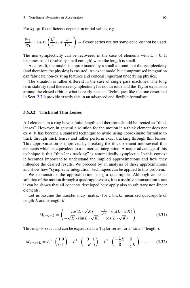
Let us assume the transfer map (matrix) for a thick, linearized quadrupole of
length L and strength K:
M s→s+L =
cos(L ·
√
K)
1
√
K
· sin(L ·
√
K)
−
√
K · sin(L ·
√
K) cos(L ·
√
K)
(3.31)
This map is exact and can be expanded as a Taylor series for a “small” length L:
M s→s+L = L
0
·
1 0
0 1
+ L
1
·
0 1
−K 0
+ L
2
·
−
1
2 K 0
0 −
1
2 K
+ . . .
(3.32)
65
For k 2 = 0 coefficients depend on initial values, e.g.:
∂y 2
∂y 1
= 1 + k 2
L 2
4
x 1 +
L 3
12x 1
→ Power series are not symplectic, cannot be used
The non-symplecticity can be recovered in the case of elements with L = 0. It
becomes small (probably small enough) when the length is small.
As a result, the model is approximated by a small amount, but the symplecticity
(and therefore the physics) is ensured. An exact model but compromised integration
can fabricate non-existing features and conceal important underlying physics.
The situation is rather different in the case of single pass machines. The long
term stability (and therefore symplecticity) is not an issue and the Taylor expansion
around the closed orbit is what is really needed. Techniques like the one described
in Sect. 3.7.6 provide exactly this in an advanced and flexible formalism.
3.6.3.2 Thick and Thin Lenses
All elements in a ring have a finite length and therefore should be treated as “thick
lenses”. However, in general a solution for the motion in a thick element does not
exist. It has become a standard technique to avoid using approximate formulae to
track through thick lenses and rather perform exact tracking through thin lenses.
This approximation is improved by breaking the thick element into several thin
elements which is equivalent to a numerical integration. A major advantage of this
technique is that “thin lens tracking” is automatically symplectic. In this context
it becomes important to understand the implied approximations and how they
influence the desired results. We proceed by an analysis of these approximations
and show how “symplectic integration” techniques can be applied to this problem.
We demonstrate the approximation using a quadrupole. Although an exact
solution of the motion through a quadrupole exists, it is a useful demonstration since
it can be shown that all concepts developed here apply also to arbitrary non-linear
elements.
Let us assume the transfer map (matrix) for a thick, linearized quadrupole of
length L and strength K:
M s→s+L =
cos(L ·
√
K)
1
√
K
· sin(L ·
√
K)
−
√
K · sin(L ·
√
K) cos(L ·
√
K)
(3.31)
This map is exact and can be expanded as a Taylor series for a “small” length L:
M s→s+L = L
0
·
1 0
0 1
+ L
1
·
0 1
−K 0
+ L
2
·
−
1
2 K 0
0 −
1
2 K
+ . . .
(3.32)