

120
E. Metral et al.
4.3.1 Longitudinal
The most fundamental longitudinal instability encountered in circular accelerators is
called the Robinson instability. The (Radio-Frequency) RF frequency accelerating
cavities in a circular accelerator are tuned so that the resonant frequency of the
fundamental mode is very close to an integral multiple of the revolution frequency
of the beam. This necessarily means that the wake field excited by the beam in the
cavities contains a major frequency component near a multiple of the revolution
frequency. The exact value of the resonant frequency relative to the multiple of the
revolution frequency is of critical importance for the stability of the beam. Above
the transition energy, the beam will be unstable if the resonant frequency is slightly
above it and stable if slightly below. This is the opposite below transition. This
instability mechanism was first analyzed by Robinson [56]. Physically, the Robinson
instability comes from the fact that the revolution frequency of an off-momentum
beam is not given by the on-momentum revolution frequency, but by a quantity
slightly different, depending on both the slip factor and the energy deviation.
Let’s assume in the following that the Robinson criterion is met. A bunch is
longitudinally stable if the longitudinal profile observed at a wall-current monitor is
constant turn after turn and it is unstable if the longitudinal profile is not constant
turn after turn. In the case of instability, the way the longitudinal profile oscillates
gives some information about the type of instabilities. This was studied in detail
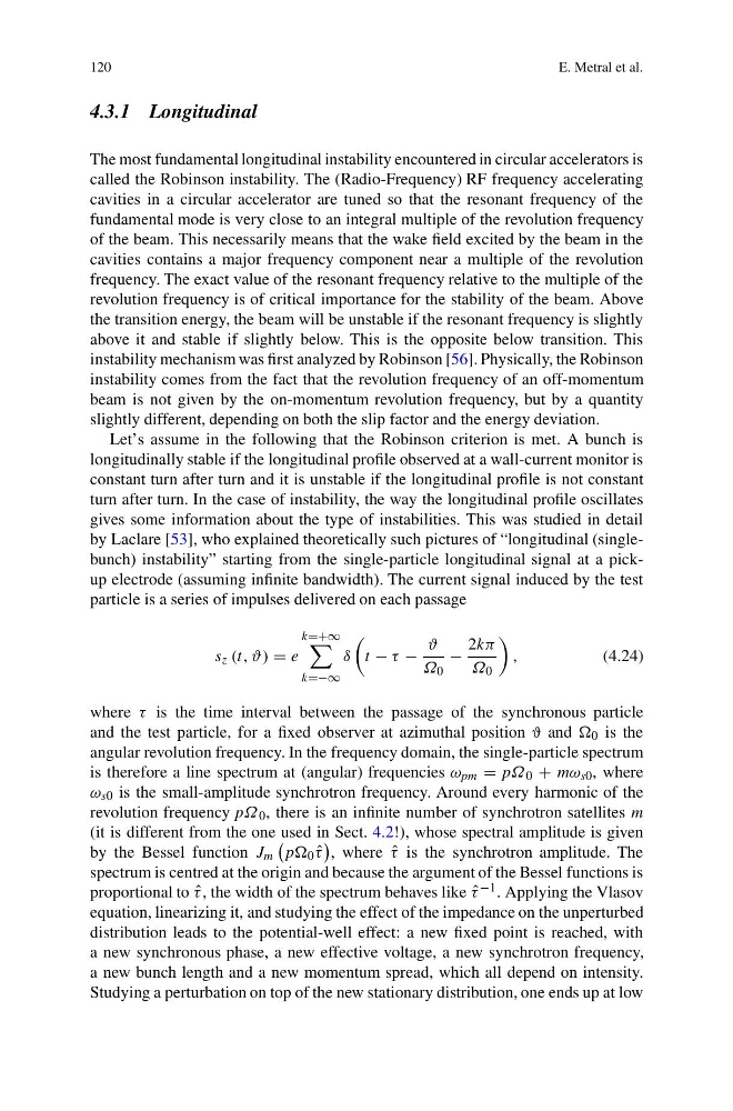
by Laclare [53], who explained theoretically such pictures of “longitudinal (singlebunch) instability” starting from the single-particle longitudinal signal at a pickup electrode (assuming infinite bandwidth). The current signal induced by the test
particle is a series of impulses delivered on each passage
s z (t, ϑ) = e
k=+∞
k=−∞
δ
t − τ −
ϑ
Ω 0
−
2kπ
Ω 0
,
(4.24)
where τ is the time interval between the passage of the synchronous particle
and the test particle, for a fixed observer at azimuthal position ϑ and 0 is the
angular revolution frequency. In the frequency domain, the single-particle spectrum
is therefore a line spectrum at (angular) frequencies ω pm = pΩ 0 + mω s0 , where
ω s0 is the small-amplitude synchrotron frequency. Around every harmonic of the
revolution frequency pΩ 0 , there is an infinite number of synchrotron satellites m
(it is different from the one used in Sect. 4.2!), whose spectral amplitude is given
by the Bessel function J m
pp 0 ˆ
τ
, where ˆ
τ is the synchrotron amplitude. The
spectrum is centred at the origin and because the argument of the Bessel functions is
proportional to ˆ
τ , the width of the spectrum behaves like ˆ
τ −1 . Applying the Vlasov
equation, linearizing it, and studying the effect of the impedance on the unperturbed
distribution leads to the potential-well effect: a new fixed point is reached, with
a new synchronous phase, a new effective voltage, a new synchrotron frequency,
a new bunch length and a new momentum spread, which all depend on intensity.
Studying a perturbation on top of the new stationary distribution, one ends up at low
E. Metral et al.
4.3.1 Longitudinal
The most fundamental longitudinal instability encountered in circular accelerators is
called the Robinson instability. The (Radio-Frequency) RF frequency accelerating
cavities in a circular accelerator are tuned so that the resonant frequency of the
fundamental mode is very close to an integral multiple of the revolution frequency
of the beam. This necessarily means that the wake field excited by the beam in the
cavities contains a major frequency component near a multiple of the revolution
frequency. The exact value of the resonant frequency relative to the multiple of the
revolution frequency is of critical importance for the stability of the beam. Above
the transition energy, the beam will be unstable if the resonant frequency is slightly
above it and stable if slightly below. This is the opposite below transition. This
instability mechanism was first analyzed by Robinson [56]. Physically, the Robinson
instability comes from the fact that the revolution frequency of an off-momentum
beam is not given by the on-momentum revolution frequency, but by a quantity
slightly different, depending on both the slip factor and the energy deviation.
Let’s assume in the following that the Robinson criterion is met. A bunch is
longitudinally stable if the longitudinal profile observed at a wall-current monitor is
constant turn after turn and it is unstable if the longitudinal profile is not constant
turn after turn. In the case of instability, the way the longitudinal profile oscillates
gives some information about the type of instabilities. This was studied in detail
by Laclare [53], who explained theoretically such pictures of “longitudinal (singlebunch) instability” starting from the single-particle longitudinal signal at a pickup electrode (assuming infinite bandwidth). The current signal induced by the test
particle is a series of impulses delivered on each passage
s z (t, ϑ) = e
k=+∞
k=−∞
δ
t − τ −
ϑ
Ω 0
−
2kπ
Ω 0
,
(4.24)
where τ is the time interval between the passage of the synchronous particle
and the test particle, for a fixed observer at azimuthal position ϑ and 0 is the
angular revolution frequency. In the frequency domain, the single-particle spectrum
is therefore a line spectrum at (angular) frequencies ω pm = pΩ 0 + mω s0 , where
ω s0 is the small-amplitude synchrotron frequency. Around every harmonic of the
revolution frequency pΩ 0 , there is an infinite number of synchrotron satellites m
(it is different from the one used in Sect. 4.2!), whose spectral amplitude is given
by the Bessel function J m
pp 0 ˆ
τ
, where ˆ
τ is the synchrotron amplitude. The
spectrum is centred at the origin and because the argument of the Bessel functions is
proportional to ˆ
τ , the width of the spectrum behaves like ˆ
τ −1 . Applying the Vlasov
equation, linearizing it, and studying the effect of the impedance on the unperturbed
distribution leads to the potential-well effect: a new fixed point is reached, with
a new synchronous phase, a new effective voltage, a new synchrotron frequency,
a new bunch length and a new momentum spread, which all depend on intensity.
Studying a perturbation on top of the new stationary distribution, one ends up at low