

100
W. Herr and E. Forest
−1.5 −1 −0.5
0.5
1
1.5
12.55
12.6
12.65
12.7
Φ+π/2
J/h
μ/2π = 0.31
−1.5 −1 −0.5
0.5
1
1.5
49.8
49.9
50.1
50.2
J/h
Φ + π/2
μ/2π = 0.31
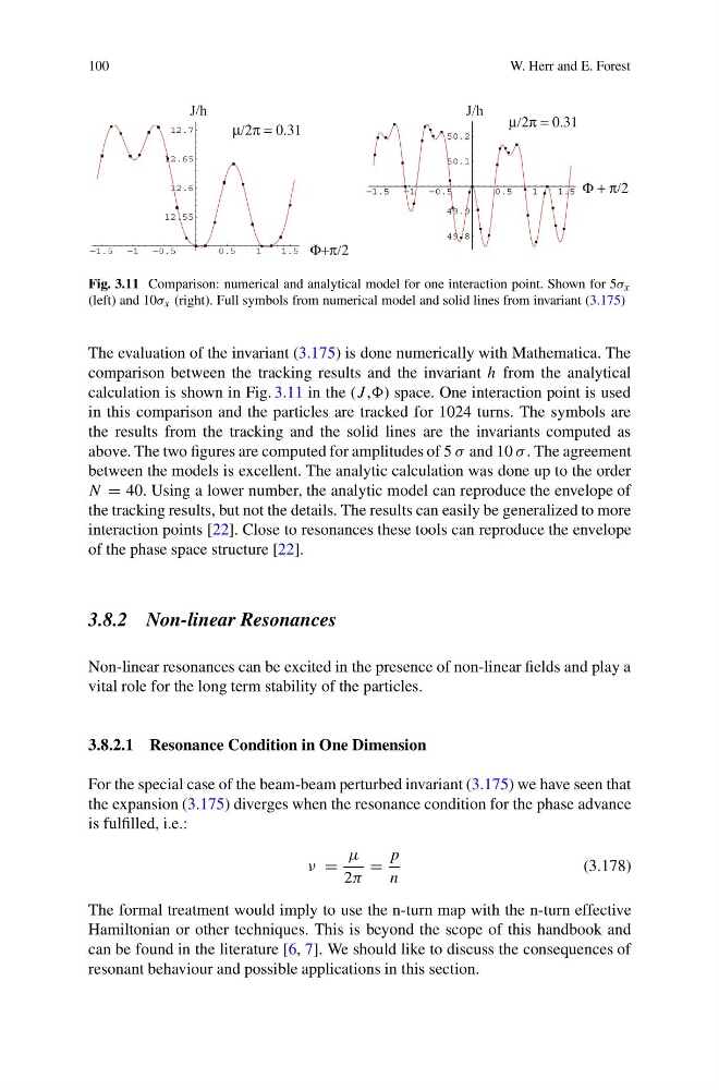
Fig. 3.11 Comparison: numerical and analytical model for one interaction point. Shown for 5σ x
(left) and 10σ x (right). Full symbols from numerical model and solid lines from invariant (3.175)
The evaluation of the invariant (3.175) is done numerically with Mathematica. The
comparison between the tracking results and the invariant h from the analytical
calculation is shown in Fig. 3.11 in the (J ,) space. One interaction point is used
in this comparison and the particles are tracked for 1024 turns. The symbols are
the results from the tracking and the solid lines are the invariants computed as
above. The two figures are computed for amplitudes of 5 σ and 10 σ . The agreement
between the models is excellent. The analytic calculation was done up to the order
N = 40. Using a lower number, the analytic model can reproduce the envelope of
the tracking results, but not the details. The results can easily be generalized to more
interaction points [22]. Close to resonances these tools can reproduce the envelope
of the phase space structure [22].
3.8.2 Non-linear Resonances
Non-linear resonances can be excited in the presence of non-linear fields and play a
vital role for the long term stability of the particles.
3.8.2.1 Resonance Condition in One Dimension
For the special case of the beam-beam perturbed invariant (3.175) we have seen that
the expansion (3.175) diverges when the resonance condition for the phase advance
is fulfilled, i.e.:
ν =
μ
2π
=
p
n
(3.178)
The formal treatment would imply to use the n-turn map with the n-turn effective
Hamiltonian or other techniques. This is beyond the scope of this handbook and
can be found in the literature [6, 7]. We should like to discuss the consequences of
resonant behaviour and possible applications in this section.
W. Herr and E. Forest
−1.5 −1 −0.5
0.5
1
1.5
12.55
12.6
12.65
12.7
Φ+π/2
J/h
μ/2π = 0.31
−1.5 −1 −0.5
0.5
1
1.5
49.8
49.9
50.1
50.2
J/h
Φ + π/2
μ/2π = 0.31
Fig. 3.11 Comparison: numerical and analytical model for one interaction point. Shown for 5σ x
(left) and 10σ x (right). Full symbols from numerical model and solid lines from invariant (3.175)
The evaluation of the invariant (3.175) is done numerically with Mathematica. The
comparison between the tracking results and the invariant h from the analytical
calculation is shown in Fig. 3.11 in the (J ,) space. One interaction point is used
in this comparison and the particles are tracked for 1024 turns. The symbols are
the results from the tracking and the solid lines are the invariants computed as
above. The two figures are computed for amplitudes of 5 σ and 10 σ . The agreement
between the models is excellent. The analytic calculation was done up to the order
N = 40. Using a lower number, the analytic model can reproduce the envelope of
the tracking results, but not the details. The results can easily be generalized to more
interaction points [22]. Close to resonances these tools can reproduce the envelope
of the phase space structure [22].
3.8.2 Non-linear Resonances
Non-linear resonances can be excited in the presence of non-linear fields and play a
vital role for the long term stability of the particles.
3.8.2.1 Resonance Condition in One Dimension
For the special case of the beam-beam perturbed invariant (3.175) we have seen that
the expansion (3.175) diverges when the resonance condition for the phase advance
is fulfilled, i.e.:
ν =
μ
2π
=
p
n
(3.178)
The formal treatment would imply to use the n-turn map with the n-turn effective
Hamiltonian or other techniques. This is beyond the scope of this handbook and
can be found in the literature [6, 7]. We should like to discuss the consequences of
resonant behaviour and possible applications in this section.