

98
W. Herr and E. Forest
with
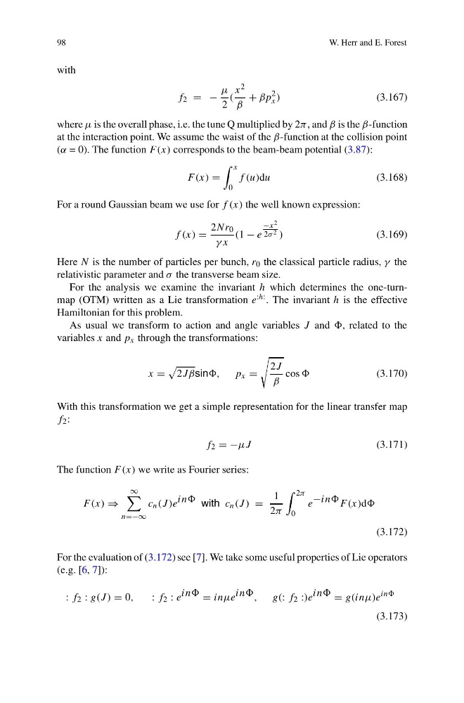
f 2 = −
μ
2
(
x 2
β
+ βp
2
x )
(3.167)
where μ is the overall phase, i.e. the tune Q multiplied by 2π, and β is the β-function
at the interaction point. We assume the waist of the β-function at the collision point
(α = 0). The function F (x) corresponds to the beam-beam potential (3.87):
F (x) =
x
0
f (u)du
(3.168)
For a round Gaussian beam we use for f (x) the well known expression:
f (x) =
2Nr 0
γ x
(1 − e
−x 2
2σ 2 )
(3.169)
Here N is the number of particles per bunch, r 0 the classical particle radius, γ the
relativistic parameter and σ the transverse beam size.
For the analysis we examine the invariant h which determines the one-turnmap (OTM) written as a Lie transformation e :h: . The invariant h is the effective
Hamiltonian for this problem.
As usual we transform to action and angle variables J and , related to the
variables x and p x through the transformations:
x =
2Jβsin, p x =
2J
β
cos
(3.170)
With this transformation we get a simple representation for the linear transfer map
f 2 :
f 2 = −μJ
(3.171)
The function F (x) we write as Fourier series:
F (x) ⇒
∞
n=−∞
c n (J )e inn with c n (J ) =
1
2π
2π
0
e −inn F (x)d
(3.172)
For the evaluation of (3.172) see [7]. We take some useful properties of Lie operators
(e.g. [6, 7]):
: f 2 : g(J ) = 0,
: f 2 : e in = inμe inn , g(: f 2 :)e inn = g(inμ)e
inn
(3.173)
W. Herr and E. Forest
with
f 2 = −
μ
2
(
x 2
β
+ βp
2
x )
(3.167)
where μ is the overall phase, i.e. the tune Q multiplied by 2π, and β is the β-function
at the interaction point. We assume the waist of the β-function at the collision point
(α = 0). The function F (x) corresponds to the beam-beam potential (3.87):
F (x) =
x
0
f (u)du
(3.168)
For a round Gaussian beam we use for f (x) the well known expression:
f (x) =
2Nr 0
γ x
(1 − e
−x 2
2σ 2 )
(3.169)
Here N is the number of particles per bunch, r 0 the classical particle radius, γ the
relativistic parameter and σ the transverse beam size.
For the analysis we examine the invariant h which determines the one-turnmap (OTM) written as a Lie transformation e :h: . The invariant h is the effective
Hamiltonian for this problem.
As usual we transform to action and angle variables J and , related to the
variables x and p x through the transformations:
x =
2Jβsin, p x =
2J
β
cos
(3.170)
With this transformation we get a simple representation for the linear transfer map
f 2 :
f 2 = −μJ
(3.171)
The function F (x) we write as Fourier series:
F (x) ⇒
∞
n=−∞
c n (J )e inn with c n (J ) =
1
2π
2π
0
e −inn F (x)d
(3.172)
For the evaluation of (3.172) see [7]. We take some useful properties of Lie operators
(e.g. [6, 7]):
: f 2 : g(J ) = 0,
: f 2 : e in = inμe inn , g(: f 2 :)e inn = g(inμ)e
inn
(3.173)