

3 Non-linear Dynamics in Accelerators
91
Using the same procedure for f (x) = x −1 one obtains:
(x, 1, 0, 0, ..)
−1
= (
1
x
. −
1
x 2 ,
2
x 3 , . . .)
(3.159)
For the function we have used before (3.145) :
f (x) = x
2
+
1
x
(3.160)
and using (adding!) the expressions (3.156) and (3.159) one has:
(f 0 , f
, f
, f
) = (x
2
+
1
x
, 2x −
1
x 2 , 2 +
2
x 3 , ..)
(3.161)
3.7.6.5 Automatic Differentiation: More Variables
It can be extended to more variables x, y and a function f (x, y):
x = (a, 1, 0, 0, 0 . . .)
(3.162)
y = (b, 0, 1, 0, 0 . . .)
(3.163)
and get (with more complicated multiplication rules):
f ((x + dx), y + dy)) =
f,
∂f
∂x
,
∂f
∂y
,
∂ 2 f
∂x 2 ,
∂ 2 f
∂x∂y
, . . .
(x, y)
(3.164)
3.7.6.6 Differential Algebra: Applications to Accelerators
Of course it is not the purpose of these tools to compute analytical expressions
for the derivatives, the examples were used to demonstrate the techniques. The
application of these techniques (i.e. Truncated Power Series Algebra [6, 21]) is
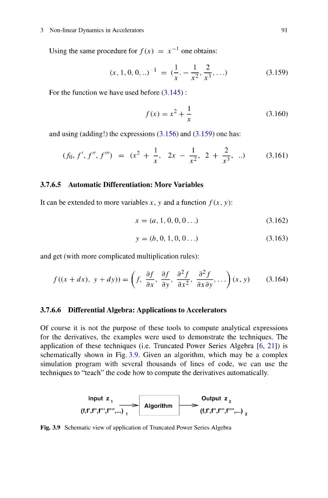
schematically shown in Fig. 3.9. Given an algorithm, which may be a complex
simulation program with several thousands of lines of code, we can use the
techniques to “teach” the code how to compute the derivatives automatically.
Algorithm
(f,f’,f”,f”’,f””,...)
(f,f’,f”,f”’,f””,...) 2
1
2
1
Input z
Output z
Fig. 3.9 Schematic view of application of Truncated Power Series Algebra
91
Using the same procedure for f (x) = x −1 one obtains:
(x, 1, 0, 0, ..)
−1
= (
1
x
. −
1
x 2 ,
2
x 3 , . . .)
(3.159)
For the function we have used before (3.145) :
f (x) = x
2
+
1
x
(3.160)
and using (adding!) the expressions (3.156) and (3.159) one has:
(f 0 , f
, f
, f
) = (x
2
+
1
x
, 2x −
1
x 2 , 2 +
2
x 3 , ..)
(3.161)
3.7.6.5 Automatic Differentiation: More Variables
It can be extended to more variables x, y and a function f (x, y):
x = (a, 1, 0, 0, 0 . . .)
(3.162)
y = (b, 0, 1, 0, 0 . . .)
(3.163)
and get (with more complicated multiplication rules):
f ((x + dx), y + dy)) =
f,
∂f
∂x
,
∂f
∂y
,
∂ 2 f
∂x 2 ,
∂ 2 f
∂x∂y
, . . .
(x, y)
(3.164)
3.7.6.6 Differential Algebra: Applications to Accelerators
Of course it is not the purpose of these tools to compute analytical expressions
for the derivatives, the examples were used to demonstrate the techniques. The
application of these techniques (i.e. Truncated Power Series Algebra [6, 21]) is
schematically shown in Fig. 3.9. Given an algorithm, which may be a complex
simulation program with several thousands of lines of code, we can use the
techniques to “teach” the code how to compute the derivatives automatically.
Algorithm
(f,f’,f”,f”’,f””,...)
(f,f’,f”,f”’,f””,...) 2
1
2
1
Input z
Output z
Fig. 3.9 Schematic view of application of Truncated Power Series Algebra