

the residual variance. The analysis allowed to
characterize the model error without the influence of observation errors of input factors and
output variable. Thus we received the model
performance calculated in the best way in comparison with traditional RSR (RMSE-standard
deviation ratio) and NSE (Nash–Sutcliffe model
efficiency coefficient), which do not separate the
model errors from observation errors of input
factors and output variable.
Based on the received model error, the performance criteria RSR = S dif =S obs (sf. Equation 7.6) and NSE = 1–RSR
2 were calculated
anew for each of WR/HCR models. The resulting
values RSR < 0.60 and NSE > 0.65 represent
good or very good performance of the developed
models (Koch and Cherie 2013) that makes
possible to calculate with good accuracy the seasonal and long-term dynamics of WR and HCR
for all rivers in the Altai-Sayan mountain country.
Some conclusions directly follow from the
adequacy of the developed WR/HCR models:
• The proposed approach and methodology for
SAM of WR and HCR are universal and
suitable for mountain regions. For the territories free of stable snow cover in winter, it is
easy to identify other hydrological seasons
and geosystem groups and redefine model
parameters by means of SAM. Though climatic zones in the Altai-Sayan mountain
country are diverse (from forests and steppes
to glacial deserts in Table 7.1), each zone is
adequately characterized during SAM.
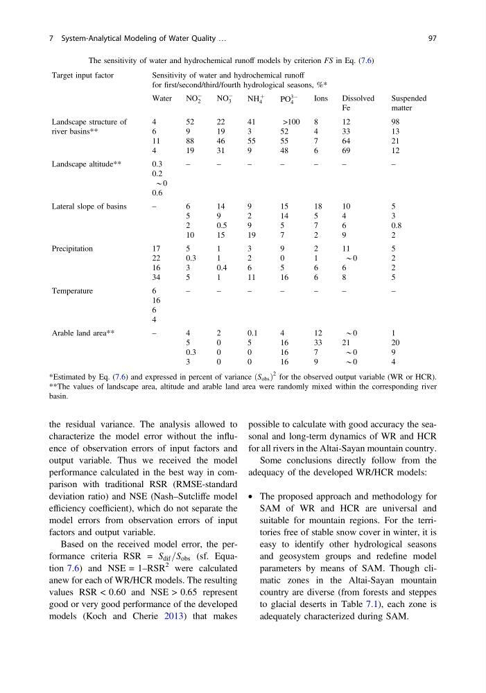
Table 7.5 The sensitivity of water and hydrochemical runoff models by criterion FS in Eq. (7.6)
Target input factor
Sensitivity of water and hydrochemical runoff
for first/second/third/fourth hydrological seasons, %*
Water
NO
À
2
NO
À
3
NH
þ
4
PO
3À
4
Ions
Dissolved
Fe
Suspended
matter
Landscape structure of
river basins**
4
6
11
4
52
9
88
19
22
19
46
31
41
3
55
9
>100
52
55
48
8
4
7
6
12
33
64
69
98
13
21
12
Landscape altitude**
0.3
0.2
*0
0.6
–
–
–
–
–
–
–
Lateral slope of basins
–
6
5
2
10
14
9
0.5
15
9
2
9
19
15
14
5
7
18
5
7
2
10
4
6
9
5
3
0.8
2
Precipitation
17
22
16
34
5
0.3
3
5
1
1
0.4
1
3
2
6
11
9
0
5
16
2
1
6
6
11
*0
6
8
5
2
2
5
Temperature
6
16
6
4
–
–
–
–
–
–
–
Arable land area**
–
4
5
0.3
3
2
0
0
0
0.1
5
0
0
4
16
16
16
12
33
7
9
*0
21
*0
*0
1
20
9
4
*Estimated by Eq. (7.6) and expressed in percent of variance S obs
ð
Þ
2 for the observed output variable (WR or HCR).
**The values of landscape area, altitude and arable land area were randomly mixed within the corresponding river
basin.
7 System-Analytical Modeling of Water Quality …
97
characterize the model error without the influence of observation errors of input factors and
output variable. Thus we received the model
performance calculated in the best way in comparison with traditional RSR (RMSE-standard
deviation ratio) and NSE (Nash–Sutcliffe model
efficiency coefficient), which do not separate the
model errors from observation errors of input
factors and output variable.
Based on the received model error, the performance criteria RSR = S dif =S obs (sf. Equation 7.6) and NSE = 1–RSR
2 were calculated
anew for each of WR/HCR models. The resulting
values RSR < 0.60 and NSE > 0.65 represent
good or very good performance of the developed
models (Koch and Cherie 2013) that makes
possible to calculate with good accuracy the seasonal and long-term dynamics of WR and HCR
for all rivers in the Altai-Sayan mountain country.
Some conclusions directly follow from the
adequacy of the developed WR/HCR models:
• The proposed approach and methodology for
SAM of WR and HCR are universal and
suitable for mountain regions. For the territories free of stable snow cover in winter, it is
easy to identify other hydrological seasons
and geosystem groups and redefine model
parameters by means of SAM. Though climatic zones in the Altai-Sayan mountain
country are diverse (from forests and steppes
to glacial deserts in Table 7.1), each zone is
adequately characterized during SAM.
Table 7.5 The sensitivity of water and hydrochemical runoff models by criterion FS in Eq. (7.6)
Target input factor
Sensitivity of water and hydrochemical runoff
for first/second/third/fourth hydrological seasons, %*
Water
NO
À
2
NO
À
3
NH
þ
4
PO
3À
4
Ions
Dissolved
Fe
Suspended
matter
Landscape structure of
river basins**
4
6
11
4
52
9
88
19
22
19
46
31
41
3
55
9
>100
52
55
48
8
4
7
6
12
33
64
69
98
13
21
12
Landscape altitude**
0.3
0.2
*0
0.6
–
–
–
–
–
–
–
Lateral slope of basins
–
6
5
2
10
14
9
0.5
15
9
2
9
19
15
14
5
7
18
5
7
2
10
4
6
9
5
3
0.8
2
Precipitation
17
22
16
34
5
0.3
3
5
1
1
0.4
1
3
2
6
11
9
0
5
16
2
1
6
6
11
*0
6
8
5
2
2
5
Temperature
6
16
6
4
–
–
–
–
–
–
–
Arable land area**
–
4
5
0.3
3
2
0
0
0
0.1
5
0
0
4
16
16
16
12
33
7
9
*0
21
*0
*0
1
20
9
4
*Estimated by Eq. (7.6) and expressed in percent of variance S obs
ð
Þ
2 for the observed output variable (WR or HCR).
**The values of landscape area, altitude and arable land area were randomly mixed within the corresponding river
basin.
7 System-Analytical Modeling of Water Quality …
97