447
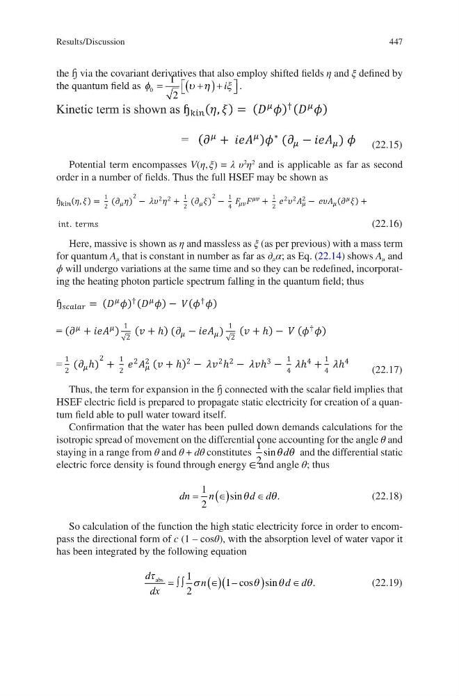
the ɧ via the covariant derivatives that also employ shifted fields η and ξ defined by
the quantum field as φ
υ η
ξ
0
1
2
=
+
(
)+
 
 
i .
(22.15)
Potential term encompasses V(η, ξ) = λ υ
2
η
2
and is applicable as far as second
order in a number of fields. Thus the full HSEF may be shown as
(22.16)
Here, massive is shown as η and massless as ξ (as per previous) with a mass term
for quantum A μ that is constant in number as far as ∂ μ α; as Eq. (22.14) shows A μ and
ϕ will undergo variations at the same time and so they can be redefined, incorporating the heating photon particle spectrum falling in the quantum field; thus
(22.17)
Thus, the term for expansion in the ɧ connected with the scalar field implies that
HSEF electric field is prepared to propagate static electricity for creation of a quantum field able to pull water toward itself.
Confirmation that the water has been pulled down demands calculations for the
isotropic spread of movement on the differential cone accounting for the angle θ and
staying in a range from θ and θ + dθ constitutes
1
2
sinθ θ
d and the differential static
electric force density is found through energy ∈ and angle θ; thus
dn
n
d d
=
∈
( )
∈
1
2
sin
.
θ
θ
(22.18)
So calculation of the function the high static electricity force in order to encompass the directional form of c (1 – cosθ), with the absorption level of water vapor it
has been integrated by the following equation
d
dx
n
d d
τ
σ
θ
θ
θ
abs
= ∫ ∫
∈
( )(
)
∈
1
2
1 – cos sin
.
(22.19)
Results/Discussion