

430
kin ,
η ξ
η
λυ η
ξ
υ
υ
µ
µ
µ
µ
µ
µ
( )= ∂
( ) −
+ ∂
( ) −
+
−
∂
1
2
1
2
1
4
1
2
2
2 2
2
2 2 2
F F
e A e A
v
v
µ µ
ξ
( ) + int.
.
terms
(21.29)
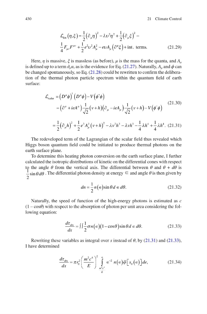
Here, η is massive, ξ is massless (as before), μ is the mass for the quanta, and A μ
is defined up to a term ∂ μ α, as is the evidence for Eq. (21.27). Naturally, A μ and ϕ can
be changed spontaneously, so Eq. (21.28) could be rewritten to confirm the deliberation of the thermal photon particle spectrum within the quantum field of earth
surface:
scalar = ( ) ( ) − ( )
= ∂ +
(
)
+
( ) ∂ −
(
)
+
(
D
D
V
ieA
v h
ieA
v h
µ
µ
µ
µ
µ
µ
φ
φ
φ φ
†
†
1
2
1
2
) ) − ( )
V φ φ
†
(21.30)
= ∂
( ) +
+
( ) −
−
−
+
1
2
1
2
1
4
1
4
2
2 2
2
2 2
3
4
4
µ
µ
λ
λ
λ
λ
h
e A v h
v h
vh
h
h . (21.31)
The redeveloped term of the Lagrangian of the scalar field thus revealed which
Higgs boson quantum field could be initiated to produce thermal photons on the
earth surface plane.
To determine this heating photon conversion on the earth surface plane, I further
calculated the isotropic distributions of kinetic on the differential cones with respect
to the angle θ from the vertical axis. The differential between θ and θ + dθ is
1
2
sinθ θ
d . The differential photon density at energy ∈ and angle θ is then given by
dn
n
d d
=
∈
( )
∈
1
2
sin
.
θ
θ
(21.32)
Naturally, the speed of function of the high-energy photons is estimated as c
(1 – cosθ) with respect to the absorption of photon per unit area considering the following equation:
d
dx
n
d d
τ
σ
θ
θ
θ
abs
= ∫ ∫
∈
( )(
)
∈
1
2
1 – cos sin
.
(21.33)
Rewriting these variables as integral over s instead of θ, by (21.31) and (21.33),
I have determined
d
dx
r
m c
E
n
s
de
m c
E
τ
π
ϕ
abs
=
∈
∈
( )
∈
( )
∞
−
∫
0
2
2 4 2
2
0
2 4
,
(21.34)
21 Climate Control
kin ,
η ξ
η
λυ η
ξ
υ
υ
µ
µ
µ
µ
µ
µ
( )= ∂
( ) −
+ ∂
( ) −
+
−
∂
1
2
1
2
1
4
1
2
2
2 2
2
2 2 2
F F
e A e A
v
v
µ µ
ξ
( ) + int.
.
terms
(21.29)
Here, η is massive, ξ is massless (as before), μ is the mass for the quanta, and A μ
is defined up to a term ∂ μ α, as is the evidence for Eq. (21.27). Naturally, A μ and ϕ can
be changed spontaneously, so Eq. (21.28) could be rewritten to confirm the deliberation of the thermal photon particle spectrum within the quantum field of earth
surface:
scalar = ( ) ( ) − ( )
= ∂ +
(
)
+
( ) ∂ −
(
)
+
(
D
D
V
ieA
v h
ieA
v h
µ
µ
µ
µ
µ
µ
φ
φ
φ φ
†
†
1
2
1
2
) ) − ( )
V φ φ
†
(21.30)
= ∂
( ) +
+
( ) −
−
−
+
1
2
1
2
1
4
1
4
2
2 2
2
2 2
3
4
4
µ
µ
λ
λ
λ
λ
h
e A v h
v h
vh
h
h . (21.31)
The redeveloped term of the Lagrangian of the scalar field thus revealed which
Higgs boson quantum field could be initiated to produce thermal photons on the
earth surface plane.
To determine this heating photon conversion on the earth surface plane, I further
calculated the isotropic distributions of kinetic on the differential cones with respect
to the angle θ from the vertical axis. The differential between θ and θ + dθ is
1
2
sinθ θ
d . The differential photon density at energy ∈ and angle θ is then given by
dn
n
d d
=
∈
( )
∈
1
2
sin
.
θ
θ
(21.32)
Naturally, the speed of function of the high-energy photons is estimated as c
(1 – cosθ) with respect to the absorption of photon per unit area considering the following equation:
d
dx
n
d d
τ
σ
θ
θ
θ
abs
= ∫ ∫
∈
( )(
)
∈
1
2
1 – cos sin
.
(21.33)
Rewriting these variables as integral over s instead of θ, by (21.31) and (21.33),
I have determined
d
dx
r
m c
E
n
s
de
m c
E
τ
π
ϕ
abs
=
∈
∈
( )
∈
( )
∞
−
∫
0
2
2 4 2
2
0
2 4
,
(21.34)
21 Climate Control