

60
3 Continuum Mechanics and Nonlinear Elasticity
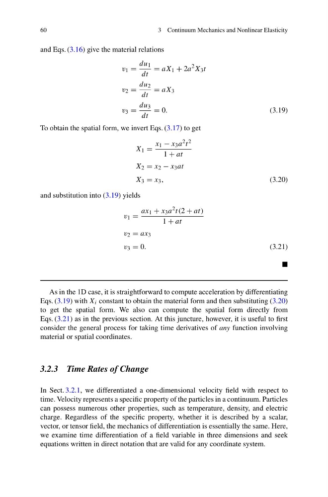
and Eqs. (3.16) give the material relations
v 1 =
du 1
dt
= aX 1 + 2a
2 X 3 t
v 2 =
du 2
dt
= aX 3
v 3 =
du 3
dt
= 0.
(3.19)
To obtain the spatial form, we invert Eqs. (3.17) to get
X 1 =
x 1 − x 3 a 2 t 2
1 + at
X 2 = x 2 − x 3 at
X 3 = x 3 ,
(3.20)
and substitution into (3.19) yields
v 1 =
ax 1 + x 3 a 2 t (2 + at)
1 + at
v 2 = ax 3
v 3 = 0.
(3.21)
As in the 1D case, it is straightforward to compute acceleration by differentiating
Eqs. (3.19) with X i constant to obtain the material form and then substituting (3.20)
to get the spatial form. We also can compute the spatial form directly from
Eqs. (3.21) as in the previous section. At this juncture, however, it is useful to first
consider the general process for taking time derivatives of any function involving
material or spatial coordinates.
3.2.3 Time Rates of Change
In Sect. 3.2.1, we differentiated a one-dimensional velocity field with respect to
time. Velocity represents a specific property of the particles in a continuum. Particles
can possess numerous other properties, such as temperature, density, and electric
charge. Regardless of the specific property, whether it is described by a scalar,
vector, or tensor field, the mechanics of differentiation is essentially the same. Here,
we examine time differentiation of a field variable in three dimensions and seek
equations written in direct notation that are valid for any coordinate system.
3 Continuum Mechanics and Nonlinear Elasticity
and Eqs. (3.16) give the material relations
v 1 =
du 1
dt
= aX 1 + 2a
2 X 3 t
v 2 =
du 2
dt
= aX 3
v 3 =
du 3
dt
= 0.
(3.19)
To obtain the spatial form, we invert Eqs. (3.17) to get
X 1 =
x 1 − x 3 a 2 t 2
1 + at
X 2 = x 2 − x 3 at
X 3 = x 3 ,
(3.20)
and substitution into (3.19) yields
v 1 =
ax 1 + x 3 a 2 t (2 + at)
1 + at
v 2 = ax 3
v 3 = 0.
(3.21)
As in the 1D case, it is straightforward to compute acceleration by differentiating
Eqs. (3.19) with X i constant to obtain the material form and then substituting (3.20)
to get the spatial form. We also can compute the spatial form directly from
Eqs. (3.21) as in the previous section. At this juncture, however, it is useful to first
consider the general process for taking time derivatives of any function involving
material or spatial coordinates.
3.2.3 Time Rates of Change
In Sect. 3.2.1, we differentiated a one-dimensional velocity field with respect to
time. Velocity represents a specific property of the particles in a continuum. Particles
can possess numerous other properties, such as temperature, density, and electric
charge. Regardless of the specific property, whether it is described by a scalar,
vector, or tensor field, the mechanics of differentiation is essentially the same. Here,
we examine time differentiation of a field variable in three dimensions and seek
equations written in direct notation that are valid for any coordinate system.