

7.4 Examples: Remodeling in 1D
363
G
n
x (t) = [J
n (t)]
1/3 ,
n= c, e.
(7.47)
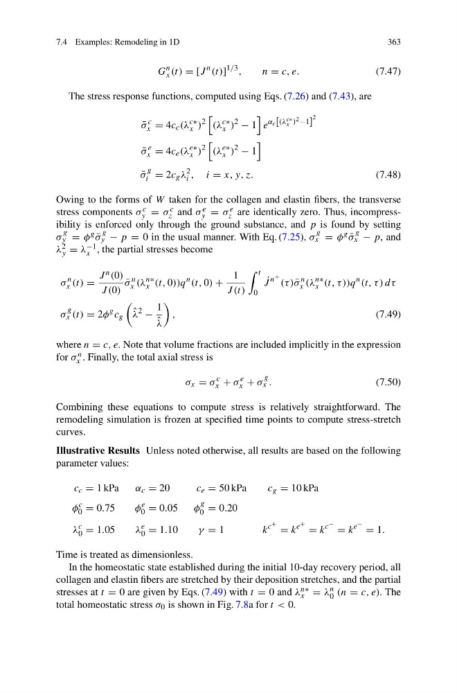
The stress response functions, computed using Eqs. (7.26) and (7.43), are
¯
σ
c
x = 4c c (λ
c∗
x )
2
(λ
c∗
x )
2
− 1
e
α c
(λ c∗
x ) 2 −1
2
¯
σ
e
x = 4c e (λ
e∗
x )
2
(λ
e∗
x )
2
− 1
¯
σ
g
i = 2c g λ
2
i , i = x, y, z.
(7.48)
Owing to the forms of W taken for the collagen and elastin fibers, the transverse
stress components σ c
y = σ c
z and σ e
y = σ e
z are identically zero. Thus, incompressibility is enforced only through the ground substance, and p is found by setting
σ
g
y = φ g ¯
σ
g
y − p = 0 in the usual manner. With Eq. (7.25), σ
g
x = φ g ¯
σ
g
x − p, and
λ 2
y = λ −1
x , the partial stresses become
σ
n
x (t) =
J n (0)
J (0)
¯
σ
n
x (λ
n∗
x (t, 0))q
n (t, 0) +
1
J (t)
t
0
˙
J
n + (τ ) ¯
σ
n
x (λ
n∗
x (t, τ ))q
n (t, τ ) dτ
σ
g
x (t) = 2φ
g c g
ˆ
λ
2
−
1
ˆ
λ
,
(7.49)
where n = c, e. Note that volume fractions are included implicitly in the expression
for σ n
x . Finally, the total axial stress is
σ x = σ
c
x + σ
e
x + σ
g
x .
(7.50)
Combining these equations to compute stress is relatively straightforward. The
remodeling simulation is frozen at specified time points to compute stress-stretch
curves.
Illustrative Results Unless noted otherwise, all results are based on the following
parameter values:
c c = 1 kPa
α c = 20
c e = 50 kPa
c g = 10 kPa
φ
c
0 = 0.75
φ
e
0 = 0.05
φ
g
0 = 0.20
λ
c
0 = 1.05
λ
e
0 = 1.10
γ = 1
k
c + = k
e + = k
c − = k
e − = 1.
Time is treated as dimensionless.
In the homeostatic state established during the initial 10-day recovery period, all
collagen and elastin fibers are stretched by their deposition stretches, and the partial
stresses at t = 0 are given by Eqs. (7.49) with t = 0 and λ n∗
x = λ n
0 (n = c, e). The
total homeostatic stress σ 0 is shown in Fig. 7.8a for t < 0.
363
G
n
x (t) = [J
n (t)]
1/3 ,
n= c, e.
(7.47)
The stress response functions, computed using Eqs. (7.26) and (7.43), are
¯
σ
c
x = 4c c (λ
c∗
x )
2
(λ
c∗
x )
2
− 1
e
α c
(λ c∗
x ) 2 −1
2
¯
σ
e
x = 4c e (λ
e∗
x )
2
(λ
e∗
x )
2
− 1
¯
σ
g
i = 2c g λ
2
i , i = x, y, z.
(7.48)
Owing to the forms of W taken for the collagen and elastin fibers, the transverse
stress components σ c
y = σ c
z and σ e
y = σ e
z are identically zero. Thus, incompressibility is enforced only through the ground substance, and p is found by setting
σ
g
y = φ g ¯
σ
g
y − p = 0 in the usual manner. With Eq. (7.25), σ
g
x = φ g ¯
σ
g
x − p, and
λ 2
y = λ −1
x , the partial stresses become
σ
n
x (t) =
J n (0)
J (0)
¯
σ
n
x (λ
n∗
x (t, 0))q
n (t, 0) +
1
J (t)
t
0
˙
J
n + (τ ) ¯
σ
n
x (λ
n∗
x (t, τ ))q
n (t, τ ) dτ
σ
g
x (t) = 2φ
g c g
ˆ
λ
2
−
1
ˆ
λ
,
(7.49)
where n = c, e. Note that volume fractions are included implicitly in the expression
for σ n
x . Finally, the total axial stress is
σ x = σ
c
x + σ
e
x + σ
g
x .
(7.50)
Combining these equations to compute stress is relatively straightforward. The
remodeling simulation is frozen at specified time points to compute stress-stretch
curves.
Illustrative Results Unless noted otherwise, all results are based on the following
parameter values:
c c = 1 kPa
α c = 20
c e = 50 kPa
c g = 10 kPa
φ
c
0 = 0.75
φ
e
0 = 0.05
φ
g
0 = 0.20
λ
c
0 = 1.05
λ
e
0 = 1.10
γ = 1
k
c + = k
e + = k
c − = k
e − = 1.
Time is treated as dimensionless.
In the homeostatic state established during the initial 10-day recovery period, all
collagen and elastin fibers are stretched by their deposition stretches, and the partial
stresses at t = 0 are given by Eqs. (7.49) with t = 0 and λ n∗
x = λ n
0 (n = c, e). The
total homeostatic stress σ 0 is shown in Fig. 7.8a for t < 0.