

6.8 Case Study: Growth of a Spherical Brain Tumor
295
R
0
J G R
2 dR =
a 0
0
J G 1 R
2 dR +
R
a 0
J G 2 R
2 dR,
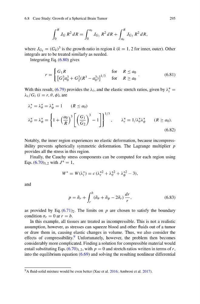
where J G k = (G k ) 3 is the growth ratio in region k (k = 1, 2 for inner, outer). Other
integrals are to be treated similarly as needed.
Integrating Eq. (6.80) gives
r =
G 1 R
for R ≤ a 0
G 3
1 a 3
0 + G 3
2 (R 3 − a 3
0 )
1/3 for R ≥ a 0
.
(6.81)
With this result, (6.79) provides the λ i , and the elastic stretch ratios, given by λ ∗
i =
λ i /G i (i = r, θ, φ), are
λ
∗
r = λ
∗
θ = λ
∗
φ = 1
(R ≤ a 0 )
λ
∗
θ = λ
∗
φ =
1 +
a 0
R
3
G 1
G 2
3
− 1
1/3
,
λ
∗
r = 1/λ
∗
θ λ
∗
φ
(R ≥ a 0 ).
(6.82)
Notably, the inner region experiences no elastic deformation, because incompressibility prevents spherically symmetric deformation. The Lagrange multiplier p
provides all the stress in this region.
Finally, the Cauchy stress components can be computed for each region using
Eqs. (6.70) 1,2 with J ∗ = 1,
W
∗
= W (λ
∗
i ) = c (λ
∗2
r + λ
∗2
θ + λ
∗2
φ − 3),
and
p = ¯
σ r +
b
r
( ¯
σ θ + ¯
σ φ − 2 ¯
σ r )
dr
r
,
(6.83)
as provided by Eq. (6.71) 2 . The limits on p are chosen to satisfy the boundary
condition σ r = 0 ar r = b.
In this example, all tissues are treated as incompressible. This is not a realistic
assumption, however, as stresses can squeeze blood and other fluids out of a tumor
or draw them in, causing elastic changes in volume. Thus, we also consider the
effects of compressibility. 9 Unfortunately, however, the problem then becomes
considerably more complicated. Finding a solution for compressible material would
entail substituting Eqs. (6.70) 1,2 , with p = 0 and stretch ratios written in terms of r,
into the equilibrium equation (6.69) and solving the resulting nonlinear differential
9 A fluid-solid mixture would be even better (Xue et al. 2016; Ambrosi et al. 2017).
295
R
0
J G R
2 dR =
a 0
0
J G 1 R
2 dR +
R
a 0
J G 2 R
2 dR,
where J G k = (G k ) 3 is the growth ratio in region k (k = 1, 2 for inner, outer). Other
integrals are to be treated similarly as needed.
Integrating Eq. (6.80) gives
r =
G 1 R
for R ≤ a 0
G 3
1 a 3
0 + G 3
2 (R 3 − a 3
0 )
1/3 for R ≥ a 0
.
(6.81)
With this result, (6.79) provides the λ i , and the elastic stretch ratios, given by λ ∗
i =
λ i /G i (i = r, θ, φ), are
λ
∗
r = λ
∗
θ = λ
∗
φ = 1
(R ≤ a 0 )
λ
∗
θ = λ
∗
φ =
1 +
a 0
R
3
G 1
G 2
3
− 1
1/3
,
λ
∗
r = 1/λ
∗
θ λ
∗
φ
(R ≥ a 0 ).
(6.82)
Notably, the inner region experiences no elastic deformation, because incompressibility prevents spherically symmetric deformation. The Lagrange multiplier p
provides all the stress in this region.
Finally, the Cauchy stress components can be computed for each region using
Eqs. (6.70) 1,2 with J ∗ = 1,
W
∗
= W (λ
∗
i ) = c (λ
∗2
r + λ
∗2
θ + λ
∗2
φ − 3),
and
p = ¯
σ r +
b
r
( ¯
σ θ + ¯
σ φ − 2 ¯
σ r )
dr
r
,
(6.83)
as provided by Eq. (6.71) 2 . The limits on p are chosen to satisfy the boundary
condition σ r = 0 ar r = b.
In this example, all tissues are treated as incompressible. This is not a realistic
assumption, however, as stresses can squeeze blood and other fluids out of a tumor
or draw them in, causing elastic changes in volume. Thus, we also consider the
effects of compressibility. 9 Unfortunately, however, the problem then becomes
considerably more complicated. Finding a solution for compressible material would
entail substituting Eqs. (6.70) 1,2 , with p = 0 and stretch ratios written in terms of r,
into the equilibrium equation (6.69) and solving the resulting nonlinear differential
9 A fluid-solid mixture would be even better (Xue et al. 2016; Ambrosi et al. 2017).