

3.5 Balance Laws
125
P in =
A 0
T
0
· v dA
0
+
V 0
b 0 · v dV
0
Q in = −
A 0
q 0 · N dA
0
+
V 0
r 0 dV
0 .
(3.186)
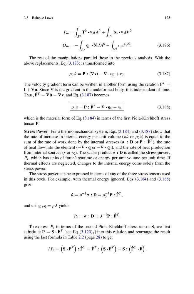
The rest of the manipulations parallel those in the previous analysis. With the
above replacements, Eq. (3.183) is transformed into
ρ 0 ˙
u = P : (∇v) − ∇ · q 0 + r 0 .
(3.187)
The velocity gradient term can be written in another form using the relation F T =
I + ∇u. Since ∇ is the gradient in the undeformed body, it is independent of time.
Thus, ˙
F T = ∇ ˙
u = ∇v, and Eq. (3.187) becomes
ρ 0 ˙
u = P : ˙
F T − ∇ · q 0 + r 0 ,
(3.188)
which is the material form of Eq. (3.184) in terms of the first Piola-Kirchhoff stress
tensor P.
Stress Power For a thermomechanical system, Eqs. (3.184) and (3.188) show that
the rate of increase in internal energy per unit volume (ρ ˙
u or ρ 0 ˙
u) is equal to the
sum of the rate of work done by the internal stresses (σ : D or P : ˙
F T ), the rate
of heat flow into the element (−∇ · q or −∇ · q 0 ), and the rate of heat production
from internal sources (r or r 0 ). The scalar product σ : D is called the stress power,
P s , which has units of force/area/time or energy per unit volume per unit time. If
thermal effects are neglected, changes to the internal energy come solely from the
stress power.
The stress power can be expressed in terms of any of the three stress tensors used
in this book. For example, with thermal energy ignored, Eqs. (3.184) and (3.188)
give
˙
u = ρ
−1
σ : D = ρ
−1
0 P : ˙
F
T ,
and using ρ 0 = ρJ yields
P s = σ : D = J
−1 P : ˙
F
T .
To express P s in terms of the second Piola-Kirchhoff stress tensor S, we first
substitute P = S · F T [see Eq. (3.120) 1 ] into this relation and rearrange the result
using the last formula in Table 2.2 (page 28) to get
J P s =
S · F
T
: ˙
F
T
= ˙
F
T
:
S · F
T
= S :
˙
F
T
· F
.
125
P in =
A 0
T
0
· v dA
0
+
V 0
b 0 · v dV
0
Q in = −
A 0
q 0 · N dA
0
+
V 0
r 0 dV
0 .
(3.186)
The rest of the manipulations parallel those in the previous analysis. With the
above replacements, Eq. (3.183) is transformed into
ρ 0 ˙
u = P : (∇v) − ∇ · q 0 + r 0 .
(3.187)
The velocity gradient term can be written in another form using the relation F T =
I + ∇u. Since ∇ is the gradient in the undeformed body, it is independent of time.
Thus, ˙
F T = ∇ ˙
u = ∇v, and Eq. (3.187) becomes
ρ 0 ˙
u = P : ˙
F T − ∇ · q 0 + r 0 ,
(3.188)
which is the material form of Eq. (3.184) in terms of the first Piola-Kirchhoff stress
tensor P.
Stress Power For a thermomechanical system, Eqs. (3.184) and (3.188) show that
the rate of increase in internal energy per unit volume (ρ ˙
u or ρ 0 ˙
u) is equal to the
sum of the rate of work done by the internal stresses (σ : D or P : ˙
F T ), the rate
of heat flow into the element (−∇ · q or −∇ · q 0 ), and the rate of heat production
from internal sources (r or r 0 ). The scalar product σ : D is called the stress power,
P s , which has units of force/area/time or energy per unit volume per unit time. If
thermal effects are neglected, changes to the internal energy come solely from the
stress power.
The stress power can be expressed in terms of any of the three stress tensors used
in this book. For example, with thermal energy ignored, Eqs. (3.184) and (3.188)
give
˙
u = ρ
−1
σ : D = ρ
−1
0 P : ˙
F
T ,
and using ρ 0 = ρJ yields
P s = σ : D = J
−1 P : ˙
F
T .
To express P s in terms of the second Piola-Kirchhoff stress tensor S, we first
substitute P = S · F T [see Eq. (3.120) 1 ] into this relation and rearrange the result
using the last formula in Table 2.2 (page 28) to get
J P s =
S · F
T
: ˙
F
T
= ˙
F
T
:
S · F
T
= S :
˙
F
T
· F
.