

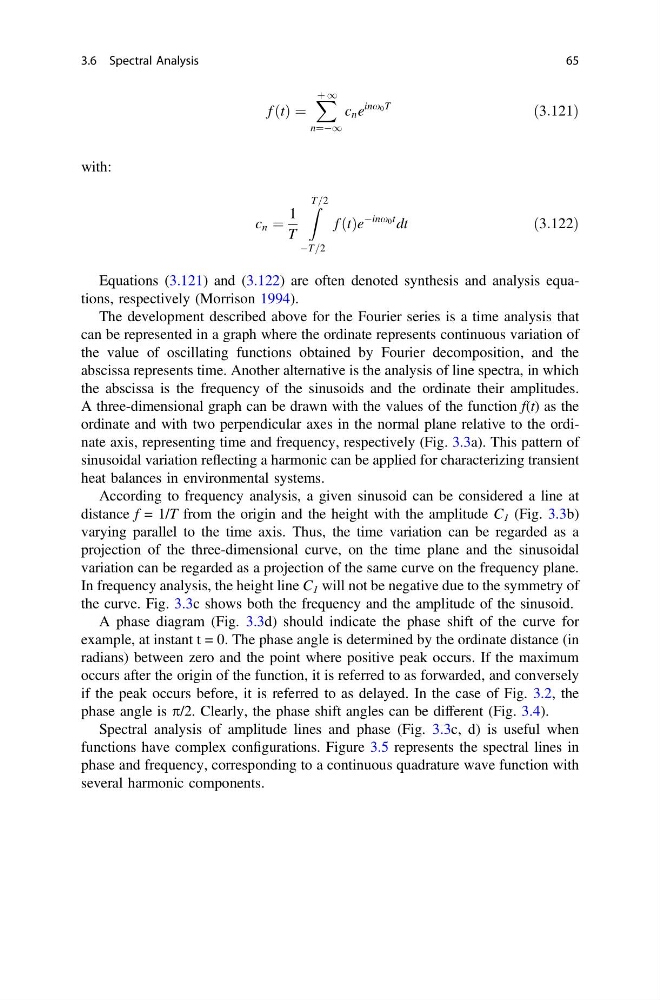
f ðtÞ ¼
X þ 1
n¼À1
c n e
inx 0 T
ð3:121Þ
with:
c n ¼
1
T
Z T=2
ÀT=2
f ðtÞe
Àinx 0 t dt
ð3:122Þ
Equations (3.121) and (3.122) are often denoted synthesis and analysis equations, respectively (Morrison 1994).
The development described above for the Fourier series is a time analysis that
can be represented in a graph where the ordinate represents continuous variation of
the value of oscillating functions obtained by Fourier decomposition, and the
abscissa represents time. Another alternative is the analysis of line spectra, in which
the abscissa is the frequency of the sinusoids and the ordinate their amplitudes.
A three-dimensional graph can be drawn with the values of the function f(t) as the
ordinate and with two perpendicular axes in the normal plane relative to the ordinate axis, representing time and frequency, respectively (Fig. 3.3a). This pattern of
sinusoidal variation reflecting a harmonic can be applied for characterizing transient
heat balances in environmental systems.
According to frequency analysis, a given sinusoid can be considered a line at
distance f = 1/T from the origin and the height with the amplitude C 1 (Fig. 3.3b)
varying parallel to the time axis. Thus, the time variation can be regarded as a
projection of the three-dimensional curve, on the time plane and the sinusoidal
variation can be regarded as a projection of the same curve on the frequency plane.
In frequency analysis, the height line C 1 will not be negative due to the symmetry of
the curve. Fig. 3.3c shows both the frequency and the amplitude of the sinusoid.
A phase diagram (Fig. 3.3d) should indicate the phase shift of the curve for
example, at instant t = 0. The phase angle is determined by the ordinate distance (in
radians) between zero and the point where positive peak occurs. If the maximum
occurs after the origin of the function, it is referred to as forwarded, and conversely
if the peak occurs before, it is referred to as delayed. In the case of Fig. 3.2, the
phase angle is p/2. Clearly, the phase shift angles can be different (Fig. 3.4).
Spectral analysis of amplitude lines and phase (Fig. 3.3c, d) is useful when
functions have complex configurations. Figure 3.5 represents the spectral lines in
phase and frequency, corresponding to a continuous quadrature wave function with
several harmonic components.
3.6 Spectral Analysis
65
X þ 1
n¼À1
c n e
inx 0 T
ð3:121Þ
with:
c n ¼
1
T
Z T=2
ÀT=2
f ðtÞe
Àinx 0 t dt
ð3:122Þ
Equations (3.121) and (3.122) are often denoted synthesis and analysis equations, respectively (Morrison 1994).
The development described above for the Fourier series is a time analysis that
can be represented in a graph where the ordinate represents continuous variation of
the value of oscillating functions obtained by Fourier decomposition, and the
abscissa represents time. Another alternative is the analysis of line spectra, in which
the abscissa is the frequency of the sinusoids and the ordinate their amplitudes.
A three-dimensional graph can be drawn with the values of the function f(t) as the
ordinate and with two perpendicular axes in the normal plane relative to the ordinate axis, representing time and frequency, respectively (Fig. 3.3a). This pattern of
sinusoidal variation reflecting a harmonic can be applied for characterizing transient
heat balances in environmental systems.
According to frequency analysis, a given sinusoid can be considered a line at
distance f = 1/T from the origin and the height with the amplitude C 1 (Fig. 3.3b)
varying parallel to the time axis. Thus, the time variation can be regarded as a
projection of the three-dimensional curve, on the time plane and the sinusoidal
variation can be regarded as a projection of the same curve on the frequency plane.
In frequency analysis, the height line C 1 will not be negative due to the symmetry of
the curve. Fig. 3.3c shows both the frequency and the amplitude of the sinusoid.
A phase diagram (Fig. 3.3d) should indicate the phase shift of the curve for
example, at instant t = 0. The phase angle is determined by the ordinate distance (in
radians) between zero and the point where positive peak occurs. If the maximum
occurs after the origin of the function, it is referred to as forwarded, and conversely
if the peak occurs before, it is referred to as delayed. In the case of Fig. 3.2, the
phase angle is p/2. Clearly, the phase shift angles can be different (Fig. 3.4).
Spectral analysis of amplitude lines and phase (Fig. 3.3c, d) is useful when
functions have complex configurations. Figure 3.5 represents the spectral lines in
phase and frequency, corresponding to a continuous quadrature wave function with
several harmonic components.
3.6 Spectral Analysis
65