

numerical methods with higher order closure equations (2nd or 3rd) or non-local
closure, are given in references such as Stull (1994).
3.6 Spectral Analysis
3.6.1 Introduction
Spectral analysis or Fourier analysis is a mathematical tool that describes data series
in terms of contributions arising from different time scales. For example, a time
series for the air temperature at a mid-latitude location will be highly variable over a
day-long period, not only because of variation in the radiative cycle but also due to
seasonal changes over a year-long period. This variation in the time domain
translates into a concomitant variation in the frequency domain, meaning that a
significant variation in time series over periods of 24 h and 8760 h (24 x 365 days)
is analogous to a significant variation in the frequencies of 1/24 h = 0.0417 h
−1 and
1/8760 = 0.000114 h
−1 . The absolute frequency is usually expressed in s
−1 or Hz.
The frequency analysis (harmonic analysis) involves representing fluctuations or
variations of time series, as summations or integrals of trigonometric functions
(sines and cosines). These harmonics are trigonometric functions in the sense that
they comprise integer multiples of the fundamental frequency determined by the
sample size of the data series. Similarly, spectral analysis can be carried out to
represent time series of an atmospheric parameter with turbulent fluctuations.
3.6.2 Fourier Series
In the nineteenth century Fourier established a paradigmatic principle “there is no
function f(x) or part of a function that cannot be expressed in trigonometric series”
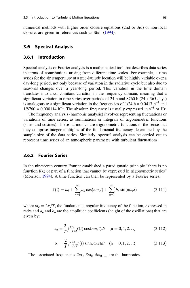
(Morrison 1994). A time function can then be represented by a Fourier series:
f t
ð Þ ¼ a 0 þ
X 1
n¼1
a n cosðnx o tÞ þ
X 1
n¼1
b n sinðnx o tÞ
ð 3:111Þ
where x 0 ¼ 2p=T, the fundamental angular frequency of the function, expressed in
rad/s and a n and b n are the amplitude coefficients (height of the oscillations) that are
given by:
a n ¼
2
T
Z T=2
ÀT=2
f ðtÞ cos nx o t
ð
Þdt ðn ¼ 0; 1; 2. . .Þ
ð 3:112Þ
b n ¼
2
T
Z T=2
ÀT=2
f ðtÞ sin nx o t
ð
Þdt ðn ¼ 0; 1; 2. . .Þ
ð 3:113Þ
The associated frequencies 2x 0, 3x 0, 4x 0, … are the harmonics.
3.5 Introduction to Turbulent Motion Equations
63
closure, are given in references such as Stull (1994).
3.6 Spectral Analysis
3.6.1 Introduction
Spectral analysis or Fourier analysis is a mathematical tool that describes data series
in terms of contributions arising from different time scales. For example, a time
series for the air temperature at a mid-latitude location will be highly variable over a
day-long period, not only because of variation in the radiative cycle but also due to
seasonal changes over a year-long period. This variation in the time domain
translates into a concomitant variation in the frequency domain, meaning that a
significant variation in time series over periods of 24 h and 8760 h (24 x 365 days)
is analogous to a significant variation in the frequencies of 1/24 h = 0.0417 h
−1 and
1/8760 = 0.000114 h
−1 . The absolute frequency is usually expressed in s
−1 or Hz.
The frequency analysis (harmonic analysis) involves representing fluctuations or
variations of time series, as summations or integrals of trigonometric functions
(sines and cosines). These harmonics are trigonometric functions in the sense that
they comprise integer multiples of the fundamental frequency determined by the
sample size of the data series. Similarly, spectral analysis can be carried out to
represent time series of an atmospheric parameter with turbulent fluctuations.
3.6.2 Fourier Series
In the nineteenth century Fourier established a paradigmatic principle “there is no
function f(x) or part of a function that cannot be expressed in trigonometric series”
(Morrison 1994). A time function can then be represented by a Fourier series:
f t
ð Þ ¼ a 0 þ
X 1
n¼1
a n cosðnx o tÞ þ
X 1
n¼1
b n sinðnx o tÞ
ð 3:111Þ
where x 0 ¼ 2p=T, the fundamental angular frequency of the function, expressed in
rad/s and a n and b n are the amplitude coefficients (height of the oscillations) that are
given by:
a n ¼
2
T
Z T=2
ÀT=2
f ðtÞ cos nx o t
ð
Þdt ðn ¼ 0; 1; 2. . .Þ
ð 3:112Þ
b n ¼
2
T
Z T=2
ÀT=2
f ðtÞ sin nx o t
ð
Þdt ðn ¼ 0; 1; 2. . .Þ
ð 3:113Þ
The associated frequencies 2x 0, 3x 0, 4x 0, … are the harmonics.
3.5 Introduction to Turbulent Motion Equations
63