

À 2v
@u 0
3 @u 0
1
@x 2
3
VI
ð3:76Þ
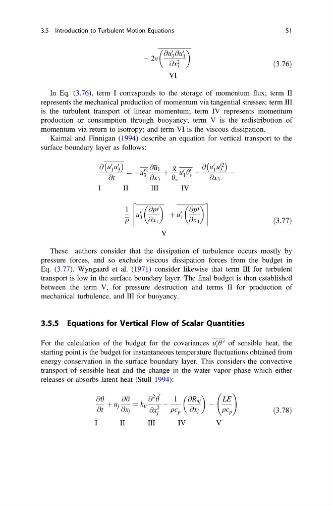
In Eq. (3.76), term I corresponds to the storage of momentum flux; term II
represents the mechanical production of momentum via tangential stresses; term III
is the turbulent transport of linear momentum; term IV represents momentum
production or consumption through buoyancy; term V is the redistribution of
momentum via return to isotropy; and term VI is the viscous dissipation.
Kaimal and Finnigan (1994) describe an equation for vertical transport to the
surface boundary layer as follows:
@ u 0
1 u 0
3
À
Á
@t
¼ Àu 02
3
@u 1
@x 3
þ
g
h v
u 0
1 h
0
v À
@ u
0
1 u
02
3
À
Á
@x 3
À
I
II
III
IV
1
q
u 0
3
@p0
@x 1
þ u 0
1
@p0
@x 3
"
#
V
ð3:77Þ
These authors consider that the dissipation of turbulence occurs mostly by
pressure forces, and so exclude viscous dissipation forces from the budget in
Eq. (3.77). Wyngaard et al. (1971) consider likewise that term III for turbulent
transport is low in the surface boundary layer. The final budget is then established
between the term V, for pressure destruction and terms II for production of
mechanical turbulence, and III for buoyancy.
3.5.5 Equations for Vertical Flow of Scalar Quantities
For the calculation of the budget for the covariances u 0
i h 0 of sensible heat, the
starting point is the budget for instantaneous temperature fluctuations obtained from
energy conservation in the surface boundary layer. This considers the convective
transport of sensible heat and the change in the water vapor phase which either
releases or absorbs latent heat (Stull 1994):
@h
@t
þ u j
@h
@x j
¼ k h
@
2 h
0
@x
2
j
À
1
qc p
@R nj
@x j
À
LE
qc p
!
I
II
III
IV
V
ð3:78Þ
3.5 Introduction to Turbulent Motion Equations
51
@u 0
3 @u 0
1
@x 2
3
VI
ð3:76Þ
In Eq. (3.76), term I corresponds to the storage of momentum flux; term II
represents the mechanical production of momentum via tangential stresses; term III
is the turbulent transport of linear momentum; term IV represents momentum
production or consumption through buoyancy; term V is the redistribution of
momentum via return to isotropy; and term VI is the viscous dissipation.
Kaimal and Finnigan (1994) describe an equation for vertical transport to the
surface boundary layer as follows:
@ u 0
1 u 0
3
À
Á
@t
¼ Àu 02
3
@u 1
@x 3
þ
g
h v
u 0
1 h
0
v À
@ u
0
1 u
02
3
À
Á
@x 3
À
I
II
III
IV
1
q
u 0
3
@p0
@x 1
þ u 0
1
@p0
@x 3
"
#
V
ð3:77Þ
These authors consider that the dissipation of turbulence occurs mostly by
pressure forces, and so exclude viscous dissipation forces from the budget in
Eq. (3.77). Wyngaard et al. (1971) consider likewise that term III for turbulent
transport is low in the surface boundary layer. The final budget is then established
between the term V, for pressure destruction and terms II for production of
mechanical turbulence, and III for buoyancy.
3.5.5 Equations for Vertical Flow of Scalar Quantities
For the calculation of the budget for the covariances u 0
i h 0 of sensible heat, the
starting point is the budget for instantaneous temperature fluctuations obtained from
energy conservation in the surface boundary layer. This considers the convective
transport of sensible heat and the change in the water vapor phase which either
releases or absorbs latent heat (Stull 1994):
@h
@t
þ u j
@h
@x j
¼ k h
@
2 h
0
@x
2
j
À
1
qc p
@R nj
@x j
À
LE
qc p
!
I
II
III
IV
V
ð3:78Þ
3.5 Introduction to Turbulent Motion Equations
51