

or:
@u i
@t
þ u j
@u i
@x j
¼ Àd i3 g þ f c e lj3 u j À
1
q
@p
@x i
þ v
@
2 u i
@x 2
j
À
@ u 0
i u 0
j
@x j
I
II
III
IV
V
VI
VII
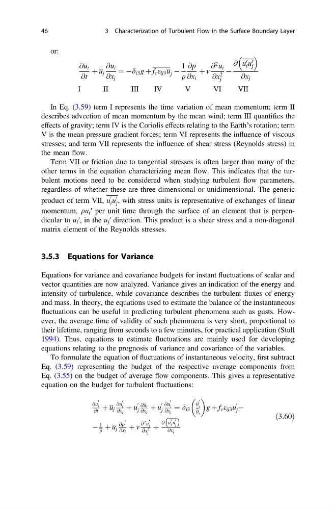
In Eq. (3.59) term I represents the time variation of mean momentum; term II
describes advection of mean momentum by the mean wind; term III quantifies the
effects of gravity; term IV is the Coriolis effects relating to the Earth’s rotation; term
V is the mean pressure gradient forces; term VI represents the influence of viscous
stresses; and term VII represents the influence of shear stress (Reynolds stress) in
the mean flow.
Term VII or friction due to tangential stresses is often larger than many of the
other terms in the equation characterizing mean flow. This indicates that the turbulent motions need to be considered when studying turbulent flow parameters,
regardless of whether these are three dimensional or unidimensional. The generic
product of term VII, u
0
i u
0
j , with stress units is representative of exchanges of linear
momentum, qu i ′ per unit time through the surface of an element that is perpendicular to u i ′, in the u j ′ direction. This product is a shear stress and a non-diagonal
matrix element of the Reynolds stresses.
3.5.3 Equations for Variance
Equations for variance and covariance budgets for instant fluctuations of scalar and
vector quantities are now analyzed. Variance gives an indication of the energy and
intensity of turbulence, while covariance describes the turbulent fluxes of energy
and mass. In theory, the equations used to estimate the balance of the instantaneous
fluctuations can be useful in predicting turbulent phenomena such as gusts. However, the average time of validity of such phenomena is very short, proportional to
their lifetime, ranging from seconds to a few minutes, for practical application (Stull
1994). Thus, equations to estimate fluctuations are mainly used for developing
equations relating to the prognosis of variance and covariance of the variables.
To formulate the equation of fluctuations of instantaneous velocity, first subtract
Eq. (3.59) representing the budget of the respective average components from
Eq. (3.55) on the budget of average flow components. This gives a representative
equation on the budget for turbulent fluctuations:
@u
0
i
@t þ u j
@u
0
i
@x j
þ u
0
j
@u i
@x j
þ u
0
j
@u
0
i
@x j
¼ d i3
h
0
v
h v
g þ f c e ij3 u
0
j À
À
1
q þ u j
@p
0
@x i
þ v
@
2 u
0
i
@x 2
j
þ
@ u
0
i u
0
j
À Á
@x j
ð3:60Þ
46
3 Characterization of Turbulent Flow in the Surface Boundary Layer
@u i
@t
þ u j
@u i
@x j
¼ Àd i3 g þ f c e lj3 u j À
1
q
@p
@x i
þ v
@
2 u i
@x 2
j
À
@ u 0
i u 0
j
@x j
I
II
III
IV
V
VI
VII
In Eq. (3.59) term I represents the time variation of mean momentum; term II
describes advection of mean momentum by the mean wind; term III quantifies the
effects of gravity; term IV is the Coriolis effects relating to the Earth’s rotation; term
V is the mean pressure gradient forces; term VI represents the influence of viscous
stresses; and term VII represents the influence of shear stress (Reynolds stress) in
the mean flow.
Term VII or friction due to tangential stresses is often larger than many of the
other terms in the equation characterizing mean flow. This indicates that the turbulent motions need to be considered when studying turbulent flow parameters,
regardless of whether these are three dimensional or unidimensional. The generic
product of term VII, u
0
i u
0
j , with stress units is representative of exchanges of linear
momentum, qu i ′ per unit time through the surface of an element that is perpendicular to u i ′, in the u j ′ direction. This product is a shear stress and a non-diagonal
matrix element of the Reynolds stresses.
3.5.3 Equations for Variance
Equations for variance and covariance budgets for instant fluctuations of scalar and
vector quantities are now analyzed. Variance gives an indication of the energy and
intensity of turbulence, while covariance describes the turbulent fluxes of energy
and mass. In theory, the equations used to estimate the balance of the instantaneous
fluctuations can be useful in predicting turbulent phenomena such as gusts. However, the average time of validity of such phenomena is very short, proportional to
their lifetime, ranging from seconds to a few minutes, for practical application (Stull
1994). Thus, equations to estimate fluctuations are mainly used for developing
equations relating to the prognosis of variance and covariance of the variables.
To formulate the equation of fluctuations of instantaneous velocity, first subtract
Eq. (3.59) representing the budget of the respective average components from
Eq. (3.55) on the budget of average flow components. This gives a representative
equation on the budget for turbulent fluctuations:
@u
0
i
@t þ u j
@u
0
i
@x j
þ u
0
j
@u i
@x j
þ u
0
j
@u
0
i
@x j
¼ d i3
h
0
v
h v
g þ f c e ij3 u
0
j À
À
1
q þ u j
@p
0
@x i
þ v
@
2 u
0
i
@x 2
j
þ
@ u
0
i u
0
j
À Á
@x j
ð3:60Þ
46
3 Characterization of Turbulent Flow in the Surface Boundary Layer