

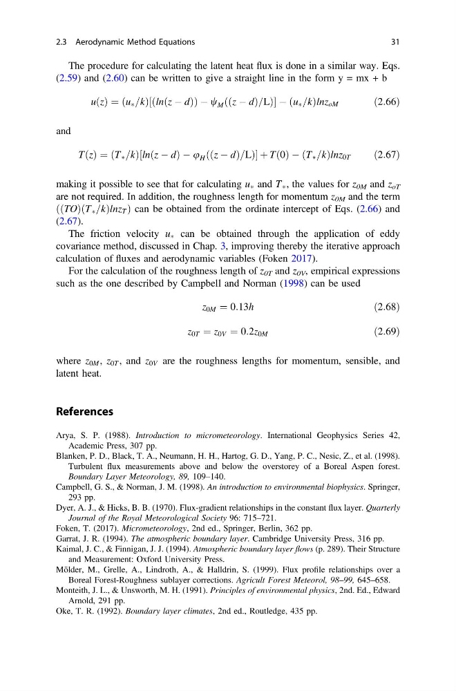
The procedure for calculating the latent heat flux is done in a similar way. Eqs.
(2.59) and (2.60) can be written to give a straight line in the form y = mx + b
u z
ð Þ ¼ u à =k
ð
Þ ln z À d
ð
Þ
ð
ÞÀ w M z À d
ð
Þ=L
ð
Þ
½
À u à =k
ð
Þlnz oM
ð2:66Þ
and
T z
ð Þ ¼ T Ã =k
ð
Þln z À d
ð
ÞÀu H z À d
ð
Þ=L
ð
Þ
½
þ T 0
ð Þ À T Ã =k
ð
Þlnz 0T
ð2:67Þ
making it possible to see that for calculating u à and T à , the values for z 0M and z oT
are not required. In addition, the roughness length for momentum z 0M and the term
TO
ð Þ T Ã =k
ð
Þlnz T
ð
Þcan be obtained from the ordinate intercept of Eqs. (2.66) and
(2.67).
The friction velocity u à can be obtained through the application of eddy
covariance method, discussed in Chap. 3, improving thereby the iterative approach
calculation of fluxes and aerodynamic variables (Foken 2017).
For the calculation of the roughness length of z 0T and z 0V , empirical expressions
such as the one described by Campbell and Norman (1998) can be used
z 0M ¼ 0:13h
ð2:68Þ
z 0T ¼ z 0V ¼ 0:2z 0M
ð2:69Þ
where z 0M , z 0T , and z 0V are the roughness lengths for momentum, sensible, and
latent heat.
References
Arya, S. P. (1988). Introduction to micrometeorology. International Geophysics Series 42,
Academic Press, 307 pp.
Blanken, P. D., Black, T. A., Neumann, H. H., Hartog, G. D., Yang, P. C., Nesic, Z., et al. (1998).
Turbulent flux measurements above and below the overstorey of a Boreal Aspen forest.
Boundary Layer Meteorology, 89, 109–140.
Campbell, G. S., & Norman, J. M. (1998). An introduction to environmental biophysics. Springer,
293 pp.
Dyer, A. J., & Hicks, B. B. (1970). Flux-gradient relationships in the constant flux layer. Quarterly
Journal of the Royal Meteorological Society 96: 715–721.
Foken, T. (2017). Micrometeorology, 2nd ed., Springer, Berlin, 362 pp.
Garrat, J. R. (1994). The atmospheric boundary layer. Cambridge University Press, 316 pp.
Kaimal, J. C., & Finnigan, J. J. (1994). Atmospheric boundary layer flows (p. 289). Their Structure
and Measurement: Oxford University Press.
Mölder, M., Grelle, A., Lindroth, A., & Halldrin, S. (1999). Flux profile relationships over a
Boreal Forest-Roughness sublayer corrections. Agricult Forest Meteorol, 98–99, 645–658.
Monteith, J. L., & Unsworth, M. H. (1991). Principles of environmental physics, 2nd. Ed., Edward
Arnold, 291 pp.
Oke, T. R. (1992). Boundary layer climates, 2nd ed., Routledge, 435 pp.
2.3 Aerodynamic Method Equations
31
(2.59) and (2.60) can be written to give a straight line in the form y = mx + b
u z
ð Þ ¼ u à =k
ð
Þ ln z À d
ð
Þ
ð
ÞÀ w M z À d
ð
Þ=L
ð
Þ
½
À u à =k
ð
Þlnz oM
ð2:66Þ
and
T z
ð Þ ¼ T Ã =k
ð
Þln z À d
ð
ÞÀu H z À d
ð
Þ=L
ð
Þ
½
þ T 0
ð Þ À T Ã =k
ð
Þlnz 0T
ð2:67Þ
making it possible to see that for calculating u à and T à , the values for z 0M and z oT
are not required. In addition, the roughness length for momentum z 0M and the term
TO
ð Þ T Ã =k
ð
Þlnz T
ð
Þcan be obtained from the ordinate intercept of Eqs. (2.66) and
(2.67).
The friction velocity u à can be obtained through the application of eddy
covariance method, discussed in Chap. 3, improving thereby the iterative approach
calculation of fluxes and aerodynamic variables (Foken 2017).
For the calculation of the roughness length of z 0T and z 0V , empirical expressions
such as the one described by Campbell and Norman (1998) can be used
z 0M ¼ 0:13h
ð2:68Þ
z 0T ¼ z 0V ¼ 0:2z 0M
ð2:69Þ
where z 0M , z 0T , and z 0V are the roughness lengths for momentum, sensible, and
latent heat.
References
Arya, S. P. (1988). Introduction to micrometeorology. International Geophysics Series 42,
Academic Press, 307 pp.
Blanken, P. D., Black, T. A., Neumann, H. H., Hartog, G. D., Yang, P. C., Nesic, Z., et al. (1998).
Turbulent flux measurements above and below the overstorey of a Boreal Aspen forest.
Boundary Layer Meteorology, 89, 109–140.
Campbell, G. S., & Norman, J. M. (1998). An introduction to environmental biophysics. Springer,
293 pp.
Dyer, A. J., & Hicks, B. B. (1970). Flux-gradient relationships in the constant flux layer. Quarterly
Journal of the Royal Meteorological Society 96: 715–721.
Foken, T. (2017). Micrometeorology, 2nd ed., Springer, Berlin, 362 pp.
Garrat, J. R. (1994). The atmospheric boundary layer. Cambridge University Press, 316 pp.
Kaimal, J. C., & Finnigan, J. J. (1994). Atmospheric boundary layer flows (p. 289). Their Structure
and Measurement: Oxford University Press.
Mölder, M., Grelle, A., Lindroth, A., & Halldrin, S. (1999). Flux profile relationships over a
Boreal Forest-Roughness sublayer corrections. Agricult Forest Meteorol, 98–99, 645–658.
Monteith, J. L., & Unsworth, M. H. (1991). Principles of environmental physics, 2nd. Ed., Edward
Arnold, 291 pp.
Oke, T. R. (1992). Boundary layer climates, 2nd ed., Routledge, 435 pp.
2.3 Aerodynamic Method Equations
31