

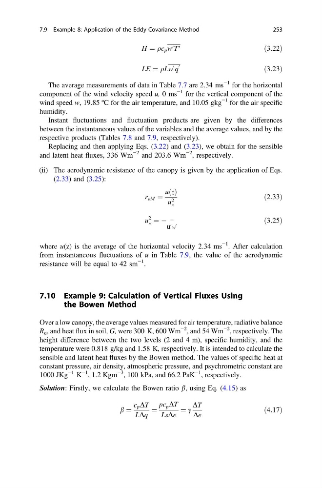
H ¼ qc p w 0 T 0
ð3:22Þ
LE ¼ qLw
0 q
0
ð3:23Þ
The average measurements of data in Table 7.7 are 2.34 ms
−1 for the horizontal
component of the wind velocity speed u, 0 ms
−1 for the vertical component of the
wind speed w, 19.85 ºC for the air temperature, and 10.05 gkg
−1 for the air specific
humidity.
Instant fluctuations and fluctuation products are given by the differences
between the instantaneous values of the variables and the average values, and by the
respective products (Tables 7.8 and 7.9, respectively).
Replacing and then applying Eqs. (3.22) and (3.23), we obtain for the sensible
and latent heat fluxes, 336 Wm
−2 and 203.6 Wm
−2 , respectively.
(ii) The aerodynamic resistance of the canopy is given by the application of Eqs.
(2.33) and (3.25):
r aM ¼
u z
ð Þ
u 2
Ã
ð2:33Þ
u
2
à ¼ À À
u
0 w
0
ð3:25Þ
where u(z) is the average of the horizontal velocity 2.34 ms
−1 . After calculation
from instantaneous fluctuations of u in Table 7.9, the value of the aerodynamic
resistance will be equal to 42 sm
−1 .
7.10 Example 9: Calculation of Vertical Fluxes Using
the Bowen Method
Over a low canopy, the average values measured for air temperature, radiative balance
R n , and heat flux in soil, G, were 300 K, 600 Wm
−2 , and 54 Wm
−2 , respectively. The
height difference between the two levels (2 and 4 m), specific humidity, and the
temperature were 0.818 g/kg and 1.58 K, respectively. It is intended to calculate the
sensible and latent heat fluxes by the Bowen method. The values of specific heat at
constant pressure, air density, atmospheric pressure, and psychrometric constant are
1000 JKg
−1 K
−1 , 1.2 Kgm
−3 , 100 kPa, and 66.2 PaK
−1 , respectively.
Solution: Firstly, we calculate the Bowen ratio b, using Eq. (4.15) as
b ¼
c p DT
LDq
¼
pc p DT
LeDe
¼ c
DT
De
ð4:17Þ
7.9 Example 8: Application of the Eddy Covariance Method
253
ð3:22Þ
LE ¼ qLw
0 q
0
ð3:23Þ
The average measurements of data in Table 7.7 are 2.34 ms
−1 for the horizontal
component of the wind velocity speed u, 0 ms
−1 for the vertical component of the
wind speed w, 19.85 ºC for the air temperature, and 10.05 gkg
−1 for the air specific
humidity.
Instant fluctuations and fluctuation products are given by the differences
between the instantaneous values of the variables and the average values, and by the
respective products (Tables 7.8 and 7.9, respectively).
Replacing and then applying Eqs. (3.22) and (3.23), we obtain for the sensible
and latent heat fluxes, 336 Wm
−2 and 203.6 Wm
−2 , respectively.
(ii) The aerodynamic resistance of the canopy is given by the application of Eqs.
(2.33) and (3.25):
r aM ¼
u z
ð Þ
u 2
Ã
ð2:33Þ
u
2
à ¼ À À
u
0 w
0
ð3:25Þ
where u(z) is the average of the horizontal velocity 2.34 ms
−1 . After calculation
from instantaneous fluctuations of u in Table 7.9, the value of the aerodynamic
resistance will be equal to 42 sm
−1 .
7.10 Example 9: Calculation of Vertical Fluxes Using
the Bowen Method
Over a low canopy, the average values measured for air temperature, radiative balance
R n , and heat flux in soil, G, were 300 K, 600 Wm
−2 , and 54 Wm
−2 , respectively. The
height difference between the two levels (2 and 4 m), specific humidity, and the
temperature were 0.818 g/kg and 1.58 K, respectively. It is intended to calculate the
sensible and latent heat fluxes by the Bowen method. The values of specific heat at
constant pressure, air density, atmospheric pressure, and psychrometric constant are
1000 JKg
−1 K
−1 , 1.2 Kgm
−3 , 100 kPa, and 66.2 PaK
−1 , respectively.
Solution: Firstly, we calculate the Bowen ratio b, using Eq. (4.15) as
b ¼
c p DT
LDq
¼
pc p DT
LeDe
¼ c
DT
De
ð4:17Þ
7.9 Example 8: Application of the Eddy Covariance Method
253