

T s:t ¼ T þ A s sin 2p=P
ð
Þ t À t m
ð
Þ
ð
Þ
ð 6:9Þ
where T is the surface temperature or mean subsurface temperature, A s and P the
amplitude and the period (e.g., daily or yearly) of the surface thermal wave,
respectively, and t m the instant when T sT ¼ T.
The solution to Eq. (6.9) with the boundary conditions such that when z = 0,
T = T s(t) and z ! ∞, T ! T is given by
T z; T
ð Þ ¼
T þ A s exp Àz=D
ð
Þsin 2p=P
ð
Þ t À t m
ð
ÞÀz=D
½
ð 6:10Þ
where D known as the damping temperature, is defined as
D ¼ ðPa=pÞ
1=2
ð6:11Þ
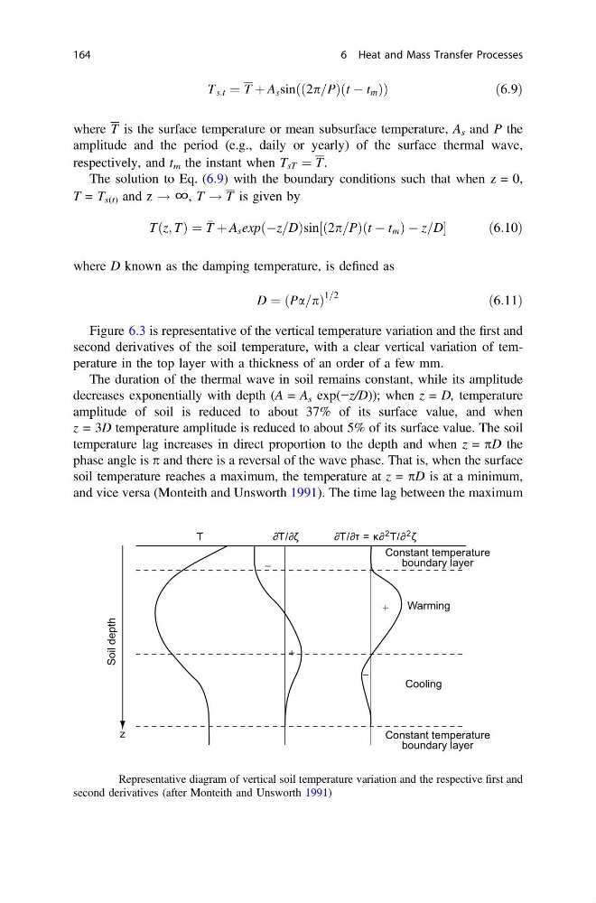
Figure 6.3 is representative of the vertical temperature variation and the first and
second derivatives of the soil temperature, with a clear vertical variation of temperature in the top layer with a thickness of an order of a few mm.
The duration of the thermal wave in soil remains constant, while its amplitude
decreases exponentially with depth (A = A s exp(−z/D)); when z = D, temperature
amplitude of soil is reduced to about 37% of its surface value, and when
z = 3D temperature amplitude is reduced to about 5% of its surface value. The soil
temperature lag increases in direct proportion to the depth and when z = pD the
phase angle is p and there is a reversal of the wave phase. That is, when the surface
soil temperature reaches a maximum, the temperature at z = pD is at a minimum,
and vice versa (Monteith and Unsworth 1991). The time lag between the maximum
Soil depth
Warming
+
+
−
−
Constant temperature
boundary layer
Constant temperature
boundary layer
Cooling
z
T
∂ Τ / ∂ ζ
∂ Τ / ∂ τ = κ ∂ 2 Τ/∂ ζ
2
Fig. 6.3 Representative diagram of vertical soil temperature variation and the respective first and
second derivatives (after Monteith and Unsworth 1991)
164
6 Heat and Mass Transfer Processes
ð
Þ t À t m
ð
Þ
ð
Þ
ð 6:9Þ
where T is the surface temperature or mean subsurface temperature, A s and P the
amplitude and the period (e.g., daily or yearly) of the surface thermal wave,
respectively, and t m the instant when T sT ¼ T.
The solution to Eq. (6.9) with the boundary conditions such that when z = 0,
T = T s(t) and z ! ∞, T ! T is given by
T z; T
ð Þ ¼
T þ A s exp Àz=D
ð
Þsin 2p=P
ð
Þ t À t m
ð
ÞÀz=D
½
ð 6:10Þ
where D known as the damping temperature, is defined as
D ¼ ðPa=pÞ
1=2
ð6:11Þ
Figure 6.3 is representative of the vertical temperature variation and the first and
second derivatives of the soil temperature, with a clear vertical variation of temperature in the top layer with a thickness of an order of a few mm.
The duration of the thermal wave in soil remains constant, while its amplitude
decreases exponentially with depth (A = A s exp(−z/D)); when z = D, temperature
amplitude of soil is reduced to about 37% of its surface value, and when
z = 3D temperature amplitude is reduced to about 5% of its surface value. The soil
temperature lag increases in direct proportion to the depth and when z = pD the
phase angle is p and there is a reversal of the wave phase. That is, when the surface
soil temperature reaches a maximum, the temperature at z = pD is at a minimum,
and vice versa (Monteith and Unsworth 1991). The time lag between the maximum
Soil depth
Warming
+
+
−
−
Constant temperature
boundary layer
Constant temperature
boundary layer
Cooling
z
T
∂ Τ / ∂ ζ
∂ Τ / ∂ τ = κ ∂ 2 Τ/∂ ζ
2
Fig. 6.3 Representative diagram of vertical soil temperature variation and the respective first and
second derivatives (after Monteith and Unsworth 1991)
164
6 Heat and Mass Transfer Processes