

78
R. Bruggemann et al.
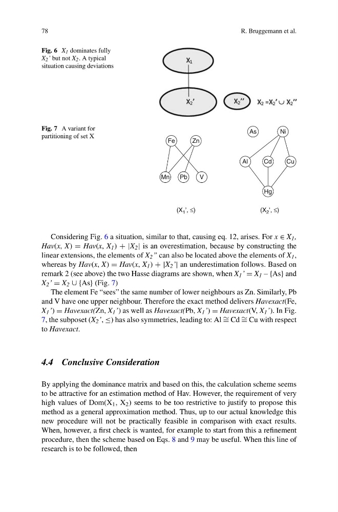
Fig. 6 X 1 dominates fully
X 2 ’ but not X 2 . A typical
situation causing deviations
Fig. 7 A variant for
partitioning of set X
Fe
Zn
As
Al
Cd
(X 2 ’, ≤)
(X 1 ’, ≤)
Hg
V
Pb
Mn
Cu
Ni
Considering Fig. 6 a situation, similar to that, causing eq. 12, arises. For x ∈ X 1 ,
Hav(x, X) = Hav(x, X 1 ) + |X 2 | is an overestimation, because by constructing the
linear extensions, the elements of X 2 ” can also be located above the elements of X 1 ,
whereas by Hav(x, X) = Hav(x, X 1 ) + |X 2 ’| an underestimation follows. Based on
remark 2 (see above) the two Hasse diagrams are shown, when X 1 ’ = X 1 – {As} and
X 2 ’ = X 2 ∪ {As} (Fig. 7)
The element Fe “sees” the same number of lower neighbours as Zn. Similarly, Pb
and V have one upper neighbour. Therefore the exact method delivers Havexact(Fe,
X 1 ’) = Havexact(Zn, X 1 ’) as well as Havexact(Pb, X 1 ’) = Havexact(V, X 1 ’). In Fig.
7, the subposet (X 2 ’, ≤) has also symmetries, leading to: Al ∼ = Cd ∼ = Cu with respect
to Havexact.
4.4 Conclusive Consideration
By applying the dominance matrix and based on this, the calculation scheme seems
to be attractive for an estimation method of Hav. However, the requirement of very
high values of Dom(X 1 , X 2 ) seems to be too restrictive to justify to propose this
method as a general approximation method. Thus, up to our actual knowledge this
new procedure will not be practically feasible in comparison with exact results.
When, however, a first check is wanted, for example to start from this a refinement
procedure, then the scheme based on Eqs. 8 and 9 may be useful. When this line of
research is to be followed, then
R. Bruggemann et al.
Fig. 6 X 1 dominates fully
X 2 ’ but not X 2 . A typical
situation causing deviations
Fig. 7 A variant for
partitioning of set X
Fe
Zn
As
Al
Cd
(X 2 ’, ≤)
(X 1 ’, ≤)
Hg
V
Pb
Mn
Cu
Ni
Considering Fig. 6 a situation, similar to that, causing eq. 12, arises. For x ∈ X 1 ,
Hav(x, X) = Hav(x, X 1 ) + |X 2 | is an overestimation, because by constructing the
linear extensions, the elements of X 2 ” can also be located above the elements of X 1 ,
whereas by Hav(x, X) = Hav(x, X 1 ) + |X 2 ’| an underestimation follows. Based on
remark 2 (see above) the two Hasse diagrams are shown, when X 1 ’ = X 1 – {As} and
X 2 ’ = X 2 ∪ {As} (Fig. 7)
The element Fe “sees” the same number of lower neighbours as Zn. Similarly, Pb
and V have one upper neighbour. Therefore the exact method delivers Havexact(Fe,
X 1 ’) = Havexact(Zn, X 1 ’) as well as Havexact(Pb, X 1 ’) = Havexact(V, X 1 ’). In Fig.
7, the subposet (X 2 ’, ≤) has also symmetries, leading to: Al ∼ = Cd ∼ = Cu with respect
to Havexact.
4.4 Conclusive Consideration
By applying the dominance matrix and based on this, the calculation scheme seems
to be attractive for an estimation method of Hav. However, the requirement of very
high values of Dom(X 1 , X 2 ) seems to be too restrictive to justify to propose this
method as a general approximation method. Thus, up to our actual knowledge this
new procedure will not be practically feasible in comparison with exact results.
When, however, a first check is wanted, for example to start from this a refinement
procedure, then the scheme based on Eqs. 8 and 9 may be useful. When this line of
research is to be followed, then