

Uncertainty in Weights for Composite Indicators Generated by Weighted Sums
53
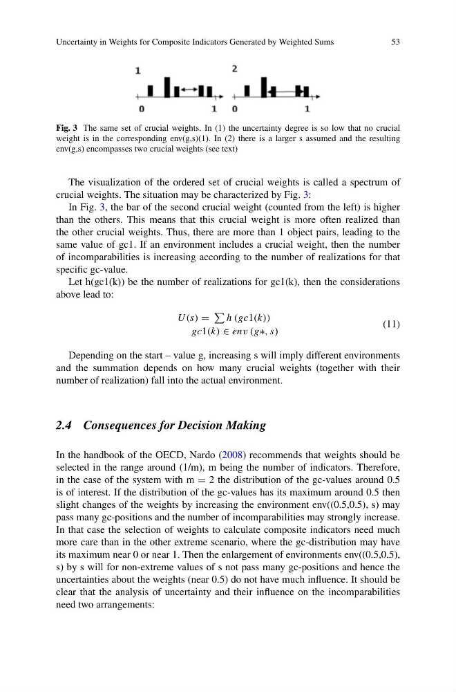
Fig. 3 The same set of crucial weights. In (1) the uncertainty degree is so low that no crucial
weight is in the corresponding env(g,s)(1). In (2) there is a larger s assumed and the resulting
env(g,s) encompasses two crucial weights (see text)
The visualization of the ordered set of crucial weights is called a spectrum of
crucial weights. The situation may be characterized by Fig. 3:
In Fig. 3, the bar of the second crucial weight (counted from the left) is higher
than the others. This means that this crucial weight is more often realized than
the other crucial weights. Thus, there are more than 1 object pairs, leading to the
same value of gc1. If an environment includes a crucial weight, then the number
of incomparabilities is increasing according to the number of realizations for that
specific gc-value.
Let h(gc1(k)) be the number of realizations for gc1(k), then the considerations
above lead to:
U(s) =
h (gc1(k))
gc1(k) ∈ env (g∗, s)
(11)
Depending on the start – value g, increasing s will imply different environments
and the summation depends on how many crucial weights (together with their
number of realization) fall into the actual environment.
2.4 Consequences for Decision Making
In the handbook of the OECD, Nardo (2008) recommends that weights should be
selected in the range around (1/m), m being the number of indicators. Therefore,
in the case of the system with m = 2 the distribution of the gc-values around 0.5
is of interest. If the distribution of the gc-values has its maximum around 0.5 then
slight changes of the weights by increasing the environment env((0.5,0.5), s) may
pass many gc-positions and the number of incomparabilities may strongly increase.
In that case the selection of weights to calculate composite indicators need much
more care than in the other extreme scenario, where the gc-distribution may have
its maximum near 0 or near 1. Then the enlargement of environments env((0.5,0.5),
s) by s will for non-extreme values of s not pass many gc-positions and hence the
uncertainties about the weights (near 0.5) do not have much influence. It should be
clear that the analysis of uncertainty and their influence on the incomparabilities
need two arrangements:
53
Fig. 3 The same set of crucial weights. In (1) the uncertainty degree is so low that no crucial
weight is in the corresponding env(g,s)(1). In (2) there is a larger s assumed and the resulting
env(g,s) encompasses two crucial weights (see text)
The visualization of the ordered set of crucial weights is called a spectrum of
crucial weights. The situation may be characterized by Fig. 3:
In Fig. 3, the bar of the second crucial weight (counted from the left) is higher
than the others. This means that this crucial weight is more often realized than
the other crucial weights. Thus, there are more than 1 object pairs, leading to the
same value of gc1. If an environment includes a crucial weight, then the number
of incomparabilities is increasing according to the number of realizations for that
specific gc-value.
Let h(gc1(k)) be the number of realizations for gc1(k), then the considerations
above lead to:
U(s) =
h (gc1(k))
gc1(k) ∈ env (g∗, s)
(11)
Depending on the start – value g, increasing s will imply different environments
and the summation depends on how many crucial weights (together with their
number of realization) fall into the actual environment.
2.4 Consequences for Decision Making
In the handbook of the OECD, Nardo (2008) recommends that weights should be
selected in the range around (1/m), m being the number of indicators. Therefore,
in the case of the system with m = 2 the distribution of the gc-values around 0.5
is of interest. If the distribution of the gc-values has its maximum around 0.5 then
slight changes of the weights by increasing the environment env((0.5,0.5), s) may
pass many gc-positions and the number of incomparabilities may strongly increase.
In that case the selection of weights to calculate composite indicators need much
more care than in the other extreme scenario, where the gc-distribution may have
its maximum near 0 or near 1. Then the enlargement of environments env((0.5,0.5),
s) by s will for non-extreme values of s not pass many gc-positions and hence the
uncertainties about the weights (near 0.5) do not have much influence. It should be
clear that the analysis of uncertainty and their influence on the incomparabilities
need two arrangements: