

Posetic Tools in the Social Sciences: A Tutorial Exposition
231
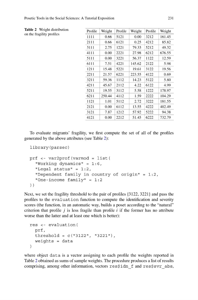
Table 2 Weight distribution
on the fragility profiles
Profile Weight Profile Weight Profile Weight
1111
0.66 5121
0.00 3212
161.45
2111
0.66 6121
0.25 4212
85.82
3111
2.75 1221
79.33 5212
49.32
4111
0.00 2221
27.98 6212
676.55
5111
0.00 3221
56.37 1122
12.59
6111
7.51 4221
145.62 2122
5.98
1211
15.48 5221
19.61 3122
19.56
2211
21.57 6221
223.55 4122
0.69
3211
59.36 1112
14.23 5122
5.80
4211
45.67 2112
4.22 6122
4.99
5211
19.55 3112
5.58 1222
178.97
6211
250.44 4112
1.59 2222
104.29
1121
1.01 5112
2.72 3222
181.55
2121
0.00 6112
13.55 4222
402.49
3121
7.87 1212
57.92 5222
94.38
4121
0.00 2212
51.45 6222
732.79
To evaluate migrants’ fragility, we first compute the set of all of the profiles
generated by the above attributes (see Table 2):
library(parsec)
prf <- var2prof(varmod = list(
"Working dynamics" = 1:6,
"Legal status" = 1:2,
"Dependent family in country of origin" = 1:2,
"One-income family" = 1:2
))
Next, we set the fragility threshold to the pair of profiles {3122, 3221} and pass the
profiles to the evaluation function to compute the identification and severity
scores (the function, in an automatic way, builds a poset according to the “natural”
criterion that profile j is less fragile than profile i if the former has no attribute
worse than the latter and at least one which is better):
res <- evaluation(
prf,
threshold = c("3122", "3221"),
weights = data
)
where object data is a vector assigning to each profile the weights reported in
Table 2 obtained as sums of sample weights. The procedure produces a list of results
comprising, among other information, vectors res$idn_f and res$svr_abs,
231
Table 2 Weight distribution
on the fragility profiles
Profile Weight Profile Weight Profile Weight
1111
0.66 5121
0.00 3212
161.45
2111
0.66 6121
0.25 4212
85.82
3111
2.75 1221
79.33 5212
49.32
4111
0.00 2221
27.98 6212
676.55
5111
0.00 3221
56.37 1122
12.59
6111
7.51 4221
145.62 2122
5.98
1211
15.48 5221
19.61 3122
19.56
2211
21.57 6221
223.55 4122
0.69
3211
59.36 1112
14.23 5122
5.80
4211
45.67 2112
4.22 6122
4.99
5211
19.55 3112
5.58 1222
178.97
6211
250.44 4112
1.59 2222
104.29
1121
1.01 5112
2.72 3222
181.55
2121
0.00 6112
13.55 4222
402.49
3121
7.87 1212
57.92 5222
94.38
4121
0.00 2212
51.45 6222
732.79
To evaluate migrants’ fragility, we first compute the set of all of the profiles
generated by the above attributes (see Table 2):
library(parsec)
prf <- var2prof(varmod = list(
"Working dynamics" = 1:6,
"Legal status" = 1:2,
"Dependent family in country of origin" = 1:2,
"One-income family" = 1:2
))
Next, we set the fragility threshold to the pair of profiles {3122, 3221} and pass the
profiles to the evaluation function to compute the identification and severity
scores (the function, in an automatic way, builds a poset according to the “natural”
criterion that profile j is less fragile than profile i if the former has no attribute
worse than the latter and at least one which is better):
res <- evaluation(
prf,
threshold = c("3122", "3221"),
weights = data
)
where object data is a vector assigning to each profile the weights reported in
Table 2 obtained as sums of sample weights. The procedure produces a list of results
comprising, among other information, vectors res$idn_f and res$svr_abs,