

1.8. THE TANGENT LINE APPROXIMATION
79
x
y
y = f (x)
a
(a, f (a))
y = f ′ (a)(x − a) + f (a)
(a, f (a))
y = f (x)
y = L(x)
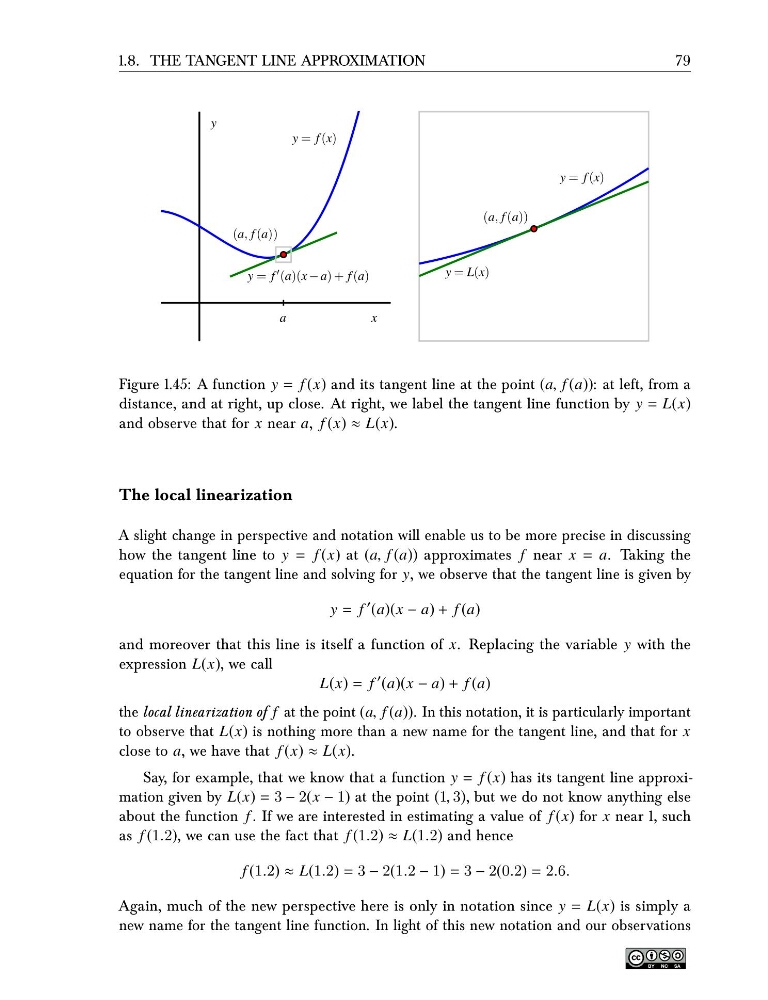
Figure 1.45: A function y = f (x) and its tangent line at the point (a, f (a)): at left, from a
distance, and at right, up close. At right, we label the tangent line function by y = L(x)
and observe that for x near a, f (x) ≈ L(x).
The local linearization
A slight change in perspective and notation will enable us to be more precise in discussing
how the tangent line to y = f (x) at (a, f (a)) approximates f near x = a. Taking the
equation for the tangent line and solving for y, we observe that the tangent line is given by
y = f
′ (a)(x − a) + f (a)
and moreover that this line is itself a function of x. Replacing the variable y with the
expression L(x), we call
L(x) = f
′ (a)(x − a) + f (a)
the local linearization of f at the point (a, f (a)). In this notation, it is particularly important
to observe that L(x) is nothing more than a new name for the tangent line, and that for x
close to a, we have that f (x) ≈ L(x).
Say, for example, that we know that a function y = f (x) has its tangent line approximation given by L(x) = 3 − 2(x − 1) at the point (1, 3), but we do not know anything else
about the function f . If we are interested in estimating a value of f (x) for x near 1, such
as f (1.2), we can use the fact that f (1.2) ≈ L(1.2) and hence
f (1.2) ≈ L(1.2) = 3 − 2(1.2 − 1) = 3 − 2(0.2) = 2.6.
Again, much of the new perspective here is only in notation since y = L(x) is simply a
new name for the tangent line function. In light of this new notation and our observations
79
x
y
y = f (x)
a
(a, f (a))
y = f ′ (a)(x − a) + f (a)
(a, f (a))
y = f (x)
y = L(x)
Figure 1.45: A function y = f (x) and its tangent line at the point (a, f (a)): at left, from a
distance, and at right, up close. At right, we label the tangent line function by y = L(x)
and observe that for x near a, f (x) ≈ L(x).
The local linearization
A slight change in perspective and notation will enable us to be more precise in discussing
how the tangent line to y = f (x) at (a, f (a)) approximates f near x = a. Taking the
equation for the tangent line and solving for y, we observe that the tangent line is given by
y = f
′ (a)(x − a) + f (a)
and moreover that this line is itself a function of x. Replacing the variable y with the
expression L(x), we call
L(x) = f
′ (a)(x − a) + f (a)
the local linearization of f at the point (a, f (a)). In this notation, it is particularly important
to observe that L(x) is nothing more than a new name for the tangent line, and that for x
close to a, we have that f (x) ≈ L(x).
Say, for example, that we know that a function y = f (x) has its tangent line approximation given by L(x) = 3 − 2(x − 1) at the point (1, 3), but we do not know anything else
about the function f . If we are interested in estimating a value of f (x) for x near 1, such
as f (1.2), we can use the fact that f (1.2) ≈ L(1.2) and hence
f (1.2) ≈ L(1.2) = 3 − 2(1.2 − 1) = 3 − 2(0.2) = 2.6.
Again, much of the new perspective here is only in notation since y = L(x) is simply a
new name for the tangent line function. In light of this new notation and our observations