

66
1.7. LIMITS, CONTINUITY, AND DIFFERENTIABILITY
-3 -2 -1
1 2 3
-3
-2
-1
1
2
3
f
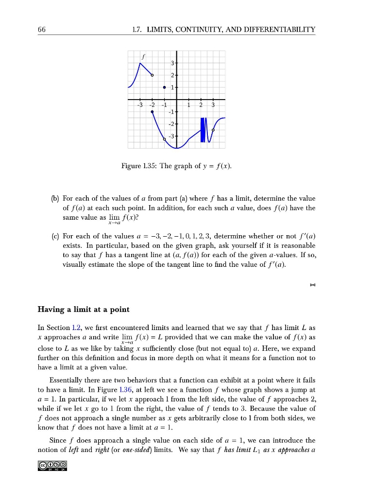
Figure 1.35: The graph of y = f (x).
(b) For each of the values of a from part (a) where f has a limit, determine the value
of f (a) at each such point. In addition, for each such a value, does f (a) have the
same value as lim
x→a
f (x)?
(c) For each of the values a = −3, −2, −1, 0, 1, 2, 3, determine whether or not f ′ (a)
exists. In particular, based on the given graph, ask yourself if it is reasonable
to say that f has a tangent line at (a, f (a)) for each of the given a-values. If so,
visually estimate the slope of the tangent line to find the value of f ′ (a).
⊲⊳
Having a limit at a point
In Section 1.2, we first encountered limits and learned that we say that f has limit L as
x approaches a and write lim
x→a
f (x) = L provided that we can make the value of f (x) as
close to L as we like by taking x sufficiently close (but not equal to) a. Here, we expand
further on this definition and focus in more depth on what it means for a function not to
have a limit at a given value.
Essentially there are two behaviors that a function can exhibit at a point where it fails
to have a limit. In Figure 1.36, at left we see a function f whose graph shows a jump at
a = 1. In particular, if we let x approach 1 from the left side, the value of f approaches 2,
while if we let x go to 1 from the right, the value of f tends to 3. Because the value of
f does not approach a single number as x gets arbitrarily close to 1 from both sides, we
know that f does not have a limit at a = 1.
Since f does approach a single value on each side of a = 1, we can introduce the
notion of left and right (or one-sided) limits. We say that f has limit L 1 as x approaches a
1.7. LIMITS, CONTINUITY, AND DIFFERENTIABILITY
-3 -2 -1
1 2 3
-3
-2
-1
1
2
3
f
Figure 1.35: The graph of y = f (x).
(b) For each of the values of a from part (a) where f has a limit, determine the value
of f (a) at each such point. In addition, for each such a value, does f (a) have the
same value as lim
x→a
f (x)?
(c) For each of the values a = −3, −2, −1, 0, 1, 2, 3, determine whether or not f ′ (a)
exists. In particular, based on the given graph, ask yourself if it is reasonable
to say that f has a tangent line at (a, f (a)) for each of the given a-values. If so,
visually estimate the slope of the tangent line to find the value of f ′ (a).
⊲⊳
Having a limit at a point
In Section 1.2, we first encountered limits and learned that we say that f has limit L as
x approaches a and write lim
x→a
f (x) = L provided that we can make the value of f (x) as
close to L as we like by taking x sufficiently close (but not equal to) a. Here, we expand
further on this definition and focus in more depth on what it means for a function not to
have a limit at a given value.
Essentially there are two behaviors that a function can exhibit at a point where it fails
to have a limit. In Figure 1.36, at left we see a function f whose graph shows a jump at
a = 1. In particular, if we let x approach 1 from the left side, the value of f approaches 2,
while if we let x go to 1 from the right, the value of f tends to 3. Because the value of
f does not approach a single number as x gets arbitrarily close to 1 from both sides, we
know that f does not have a limit at a = 1.
Since f does approach a single value on each side of a = 1, we can introduce the
notion of left and right (or one-sided) limits. We say that f has limit L 1 as x approaches a