

1.5. INTERPRETING, ESTIMATING, AND USING THE DERIVATIVE
49
20 40 60 80
100
200
300
400
y = P(t)
◦ F
min
20 40 60 80
4
8
12
16
y = P ′ (t)
◦ F/min
min
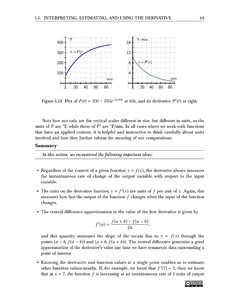
Figure 1.24: Plot of P(t) = 400 − 330e −0.03t at left, and its derivative P ′ (t) at right.
Note how not only are the vertical scales different in size, but different in units, as the
units of P are ◦ F, while those of P ′ are ◦ F/min. In all cases where we work with functions
that have an applied context, it is helpful and instructive to think carefully about units
involved and how they further inform the meaning of our computations.
Summary
In this section, we encountered the following important ideas:
• Regardless of the context of a given function y = f (x), the derivative always measures
the instantaneous rate of change of the output variable with respect to the input
variable.
• The units on the derivative function y = f ′ (x) are units of f per unit of x. Again, this
measures how fast the output of the function f changes when the input of the function
changes.
• The central difference approximation to the value of the first derivative is given by
f
′ (a) ≈
f (a + h) − f (a − h)
2h
,
and this quantity measures the slope of the secant line to y = f (x) through the
points (a − h, f (a − h)) and (a + h, f (a + h)). The central difference generates a good
approximation of the derivative’s value any time we have symmetric data surrounding a
point of interest.
• Knowing the derivative and function values at a single point enables us to estimate
other function values nearby. If, for example, we know that f ′ (7) = 2, then we know
that at x = 7, the function f is increasing at an instantaneous rate of 2 units of output
49
20 40 60 80
100
200
300
400
y = P(t)
◦ F
min
20 40 60 80
4
8
12
16
y = P ′ (t)
◦ F/min
min
Figure 1.24: Plot of P(t) = 400 − 330e −0.03t at left, and its derivative P ′ (t) at right.
Note how not only are the vertical scales different in size, but different in units, as the
units of P are ◦ F, while those of P ′ are ◦ F/min. In all cases where we work with functions
that have an applied context, it is helpful and instructive to think carefully about units
involved and how they further inform the meaning of our computations.
Summary
In this section, we encountered the following important ideas:
• Regardless of the context of a given function y = f (x), the derivative always measures
the instantaneous rate of change of the output variable with respect to the input
variable.
• The units on the derivative function y = f ′ (x) are units of f per unit of x. Again, this
measures how fast the output of the function f changes when the input of the function
changes.
• The central difference approximation to the value of the first derivative is given by
f
′ (a) ≈
f (a + h) − f (a − h)
2h
,
and this quantity measures the slope of the secant line to y = f (x) through the
points (a − h, f (a − h)) and (a + h, f (a + h)). The central difference generates a good
approximation of the derivative’s value any time we have symmetric data surrounding a
point of interest.
• Knowing the derivative and function values at a single point enables us to estimate
other function values nearby. If, for example, we know that f ′ (7) = 2, then we know
that at x = 7, the function f is increasing at an instantaneous rate of 2 units of output