

7.6. POPULATION GROWTH AND THE LOGISTIC EQUATION
443
40
80
120
160
200
3
6
9
12
15
t
P
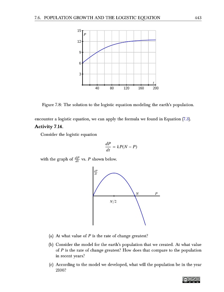
Figure 7.8: The solution to the logistic equation modeling the earth’s population.
encounter a logistic equation, we can apply the formula we found in Equation (7.3).
Activity 7.14.
Consider the logistic equation
dP
dt
= k P(N − P)
with the graph of
dP
dt vs. P shown below.
P
dP
dt
N
N/2
(a) At what value of P is the rate of change greatest?
(b) Consider the model for the earth’s population that we created. At what value
of P is the rate of change greatest? How does that compare to the population
in recent years?
(c) According to the model we developed, what will the population be in the year
2100?
443
40
80
120
160
200
3
6
9
12
15
t
P
Figure 7.8: The solution to the logistic equation modeling the earth’s population.
encounter a logistic equation, we can apply the formula we found in Equation (7.3).
Activity 7.14.
Consider the logistic equation
dP
dt
= k P(N − P)
with the graph of
dP
dt vs. P shown below.
P
dP
dt
N
N/2
(a) At what value of P is the rate of change greatest?
(b) Consider the model for the earth’s population that we created. At what value
of P is the rate of change greatest? How does that compare to the population
in recent years?
(c) According to the model we developed, what will the population be in the year
2100?