

7.6. POPULATION GROWTH AND THE LOGISTIC EQUATION
439
6.0
6.2
6.4
6.6
6.8
7.0
0.010
0.011
0.012
0.013
0.014
0.015 per capita growth rate
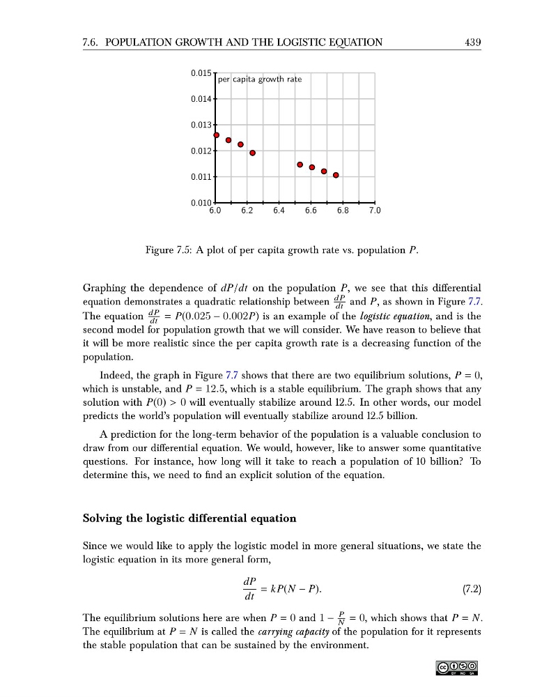
Figure 7.5: A plot of per capita growth rate vs. population P.
Graphing the dependence of dP/dt on the population P, we see that this differential
equation demonstrates a quadratic relationship between
dP
dt and P, as shown in Figure 7.7.
The equation
dP
dt = P(0.025 − 0.002P) is an example of the logistic equation, and is the
second model for population growth that we will consider. We have reason to believe that
it will be more realistic since the per capita growth rate is a decreasing function of the
population.
Indeed, the graph in Figure 7.7 shows that there are two equilibrium solutions, P = 0,
which is unstable, and P = 12.5, which is a stable equilibrium. The graph shows that any
solution with P(0) > 0 will eventually stabilize around 12.5. In other words, our model
predicts the world’s population will eventually stabilize around 12.5 billion.
A prediction for the long-term behavior of the population is a valuable conclusion to
draw from our differential equation. We would, however, like to answer some quantitative
questions. For instance, how long will it take to reach a population of 10 billion? To
determine this, we need to find an explicit solution of the equation.
Solving the logistic differential equation
Since we would like to apply the logistic model in more general situations, we state the
logistic equation in its more general form,
dP
dt
= k P(N − P).
(7.2)
The equilibrium solutions here are when P = 0 and 1 −
P
N = 0, which shows that P = N.
The equilibrium at P = N is called the carrying capacity of the population for it represents
the stable population that can be sustained by the environment.
439
6.0
6.2
6.4
6.6
6.8
7.0
0.010
0.011
0.012
0.013
0.014
0.015 per capita growth rate
Figure 7.5: A plot of per capita growth rate vs. population P.
Graphing the dependence of dP/dt on the population P, we see that this differential
equation demonstrates a quadratic relationship between
dP
dt and P, as shown in Figure 7.7.
The equation
dP
dt = P(0.025 − 0.002P) is an example of the logistic equation, and is the
second model for population growth that we will consider. We have reason to believe that
it will be more realistic since the per capita growth rate is a decreasing function of the
population.
Indeed, the graph in Figure 7.7 shows that there are two equilibrium solutions, P = 0,
which is unstable, and P = 12.5, which is a stable equilibrium. The graph shows that any
solution with P(0) > 0 will eventually stabilize around 12.5. In other words, our model
predicts the world’s population will eventually stabilize around 12.5 billion.
A prediction for the long-term behavior of the population is a valuable conclusion to
draw from our differential equation. We would, however, like to answer some quantitative
questions. For instance, how long will it take to reach a population of 10 billion? To
determine this, we need to find an explicit solution of the equation.
Solving the logistic differential equation
Since we would like to apply the logistic model in more general situations, we state the
logistic equation in its more general form,
dP
dt
= k P(N − P).
(7.2)
The equilibrium solutions here are when P = 0 and 1 −
P
N = 0, which shows that P = N.
The equilibrium at P = N is called the carrying capacity of the population for it represents
the stable population that can be sustained by the environment.