

7.5. MODELING WITH DIFFERENTIAL EQUATIONS
429
Since 5 · 10 10 cubic meters of water flow out each year 6 , then the plastic pollution leaves
the lake at the rate of
P
5 · 10 12
m 3 plastic
m 3 water
·
5 · 10
10 m 3 water
year
=
P
100
cubic meters of plastic per year.
The total rate of change of P is thus the difference between the rate at which pollution
enters the lake minus the rate at which pollution leaves the lake; that is,
dP
dt
= 1.5 · 10
3 −
P
100
=
1
100
(1.5 · 10
5 − P).
We have now found a differential equation that describes the rate at which the amount
of pollution is changing. To better understand the behavior of P(t), we now apply some of
the techniques we have recently developed.
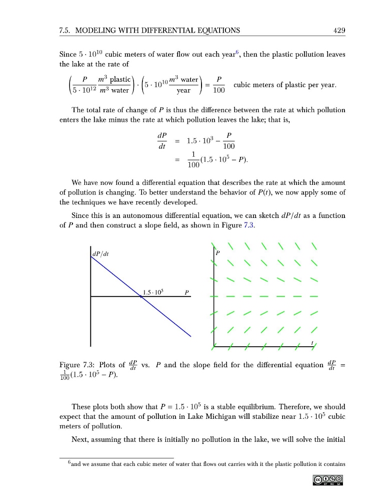
Since this is an autonomous differential equation, we can sketch dP/dt as a function
of P and then construct a slope field, as shown in Figure 7.3.
P
dP/dt
1.5 · 10 5
t
P
Figure 7.3: Plots of
dP
dt vs. P and the slope field for the differential equation
dP
dt =
1
100 (1.5 · 10 5 − P).
These plots both show that P = 1.5 · 10 5 is a stable equilibrium. Therefore, we should
expect that the amount of pollution in Lake Michigan will stabilize near 1.5 · 10 5 cubic
meters of pollution.
Next, assuming that there is initially no pollution in the lake, we will solve the initial
6 and we assume that each cubic meter of water that flows out carries with it the plastic pollution it contains
429
Since 5 · 10 10 cubic meters of water flow out each year 6 , then the plastic pollution leaves
the lake at the rate of
P
5 · 10 12
m 3 plastic
m 3 water
·
5 · 10
10 m 3 water
year
=
P
100
cubic meters of plastic per year.
The total rate of change of P is thus the difference between the rate at which pollution
enters the lake minus the rate at which pollution leaves the lake; that is,
dP
dt
= 1.5 · 10
3 −
P
100
=
1
100
(1.5 · 10
5 − P).
We have now found a differential equation that describes the rate at which the amount
of pollution is changing. To better understand the behavior of P(t), we now apply some of
the techniques we have recently developed.
Since this is an autonomous differential equation, we can sketch dP/dt as a function
of P and then construct a slope field, as shown in Figure 7.3.
P
dP/dt
1.5 · 10 5
t
P
Figure 7.3: Plots of
dP
dt vs. P and the slope field for the differential equation
dP
dt =
1
100 (1.5 · 10 5 − P).
These plots both show that P = 1.5 · 10 5 is a stable equilibrium. Therefore, we should
expect that the amount of pollution in Lake Michigan will stabilize near 1.5 · 10 5 cubic
meters of pollution.
Next, assuming that there is initially no pollution in the lake, we will solve the initial
6 and we assume that each cubic meter of water that flows out carries with it the plastic pollution it contains