

418
7.3. EULER’S METHOD
solution will most likely change over this interval. We can improve our approximation
by trying to incorporate the change in the slope over the interval.
Let’s again consider the initial value problem dy/dt = y and y(0) = 1, which we will
approximate using steps of width ∆t = 0.2. Our first interval is therefore 0 ≤ t ≤ 0.2.
At t = 0, the differential equation tells us that the slope is 1, and the approximation we
obtain from Euler’s method is that y(0.2) ≈ y 1 = 1 + 1(0.2) = 1.2.
This gives us some idea for how the slope has changed over the interval 0 ≤ t ≤ 0.2.
We know the slope at t = 0 is 1, while the slope at t = 0.2 is 1.2, trusting in the Euler’s
method approximation. We will therefore refine our estimate of the initial slope to be
the average of these two slopes; that is, we will estimate the slope to be (1 + 1.2)/2 = 1.1.
This gives the new approximation y(1) = y 1 = 1 + 1.1(0.2) = 1.22.
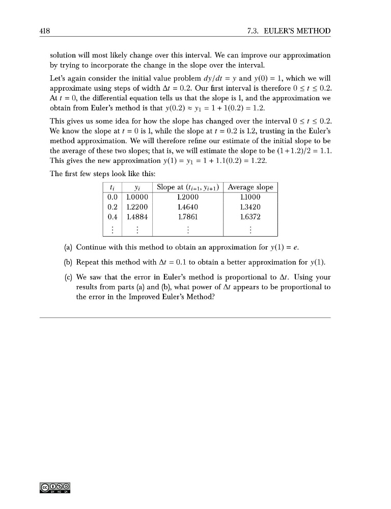
The first few steps look like this:
t i
y i
Slope at (t i+1 , y i+1 ) Average slope
0.0 1.0000
1.2000
1.1000
0.2 1.2200
1.4640
1.3420
0.4 1.4884
1.7861
1.6372
. . .
. . .
. . .
. . .
(a) Continue with this method to obtain an approximation for y(1) = e.
(b) Repeat this method with ∆t = 0.1 to obtain a better approximation for y(1).
(c) We saw that the error in Euler’s method is proportional to ∆t. Using your
results from parts (a) and (b), what power of ∆t appears to be proportional to
the error in the Improved Euler’s Method?
7.3. EULER’S METHOD
solution will most likely change over this interval. We can improve our approximation
by trying to incorporate the change in the slope over the interval.
Let’s again consider the initial value problem dy/dt = y and y(0) = 1, which we will
approximate using steps of width ∆t = 0.2. Our first interval is therefore 0 ≤ t ≤ 0.2.
At t = 0, the differential equation tells us that the slope is 1, and the approximation we
obtain from Euler’s method is that y(0.2) ≈ y 1 = 1 + 1(0.2) = 1.2.
This gives us some idea for how the slope has changed over the interval 0 ≤ t ≤ 0.2.
We know the slope at t = 0 is 1, while the slope at t = 0.2 is 1.2, trusting in the Euler’s
method approximation. We will therefore refine our estimate of the initial slope to be
the average of these two slopes; that is, we will estimate the slope to be (1 + 1.2)/2 = 1.1.
This gives the new approximation y(1) = y 1 = 1 + 1.1(0.2) = 1.22.
The first few steps look like this:
t i
y i
Slope at (t i+1 , y i+1 ) Average slope
0.0 1.0000
1.2000
1.1000
0.2 1.2200
1.4640
1.3420
0.4 1.4884
1.7861
1.6372
. . .
. . .
. . .
. . .
(a) Continue with this method to obtain an approximation for y(1) = e.
(b) Repeat this method with ∆t = 0.1 to obtain a better approximation for y(1).
(c) We saw that the error in Euler’s method is proportional to ∆t. Using your
results from parts (a) and (b), what power of ∆t appears to be proportional to
the error in the Improved Euler’s Method?