

7.3. EULER’S METHOD
415
The error in Euler’s method
Since we are approximating the solutions to an initial value problem using tangent lines,
we should expect that the error in the approximation will be less when the step size is
smaller. To explore this observation quantitatively, let’s consider the initial value problem
dy
dt
= y, y(0) = 1
whose solution we can easily find.
Consider the question posed by this initial value problem: “what function do we know
that is the same as its own derivative and has value 1 when t = 0?” It is not hard to see
that the solution is y(t) = e t . We now apply Euler’s method to approximate y(1) = e using
several values of ∆t. These approximations will be denoted by E ∆t , and these estimates
provide us a way to see how accurate Euler’s Method is.
To begin, we apply Euler’s method with a step size of ∆t = 0.2. In that case, we find
that y(1) ≈ E 0.2 = 2.4883. The error is therefore y(1) − E 0.2 = e − 2.4883 ≈ 0.2300.
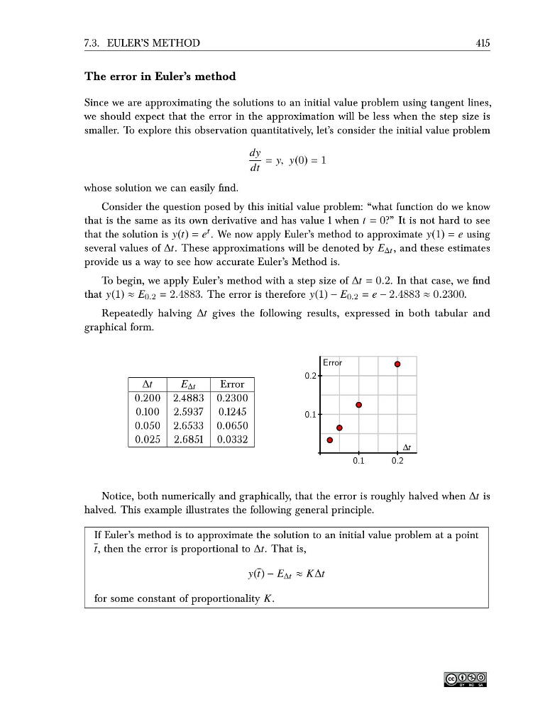
Repeatedly halving ∆t gives the following results, expressed in both tabular and
graphical form.
∆t
E ∆t
Error
0.200 2.4883 0.2300
0.100 2.5937 0.1245
0.050 2.6533 0.0650
0.025 2.6851 0.0332
0.1
0.2
0.1
0.2
Error
∆t
Notice, both numerically and graphically, that the error is roughly halved when ∆t is
halved. This example illustrates the following general principle.
If Euler’s method is to approximate the solution to an initial value problem at a point
t, then the error is proportional to ∆t. That is,
y(t) − E ∆t ≈ K∆t
for some constant of proportionality K.
415
The error in Euler’s method
Since we are approximating the solutions to an initial value problem using tangent lines,
we should expect that the error in the approximation will be less when the step size is
smaller. To explore this observation quantitatively, let’s consider the initial value problem
dy
dt
= y, y(0) = 1
whose solution we can easily find.
Consider the question posed by this initial value problem: “what function do we know
that is the same as its own derivative and has value 1 when t = 0?” It is not hard to see
that the solution is y(t) = e t . We now apply Euler’s method to approximate y(1) = e using
several values of ∆t. These approximations will be denoted by E ∆t , and these estimates
provide us a way to see how accurate Euler’s Method is.
To begin, we apply Euler’s method with a step size of ∆t = 0.2. In that case, we find
that y(1) ≈ E 0.2 = 2.4883. The error is therefore y(1) − E 0.2 = e − 2.4883 ≈ 0.2300.
Repeatedly halving ∆t gives the following results, expressed in both tabular and
graphical form.
∆t
E ∆t
Error
0.200 2.4883 0.2300
0.100 2.5937 0.1245
0.050 2.6533 0.0650
0.025 2.6851 0.0332
0.1
0.2
0.1
0.2
Error
∆t
Notice, both numerically and graphically, that the error is roughly halved when ∆t is
halved. This example illustrates the following general principle.
If Euler’s method is to approximate the solution to an initial value problem at a point
t, then the error is proportional to ∆t. That is,
y(t) − E ∆t ≈ K∆t
for some constant of proportionality K.