

382
6.5. IMPROPER INTEGRALS
y
x
f (x) =
1
√
x
1
a
y
x
f (x) =
1
√
x
1
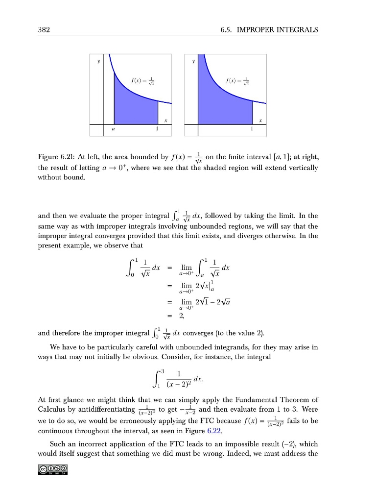
Figure 6.21: At left, the area bounded by f (x) =
1
√
x
on the finite interval [a, 1]; at right,
the result of letting a → 0 + , where we see that the shaded region will extend vertically
without bound.
and then we evaluate the proper integral
1
a
1
√
x
dx, followed by taking the limit. In the
same way as with improper integrals involving unbounded regions, we will say that the
improper integral converges provided that this limit exists, and diverges otherwise. In the
present example, we observe that
1
0
1
√
x
dx = lim
a→0 +
1
a
1
√
x
dx
= lim
a→0 +
2
√
x
1
a
= lim
a→0 +
2
√
1 − 2
√
a
= 2,
and therefore the improper integral
1
0
1
√
x
dx converges (to the value 2).
We have to be particularly careful with unbounded integrands, for they may arise in
ways that may not initially be obvious. Consider, for instance, the integral
3
1
1
(x − 2) 2 dx.
At first glance we might think that we can simply apply the Fundamental Theorem of
Calculus by antidifferentiating
1
(x−2) 2 to get −
1
x−2 and then evaluate from 1 to 3. Were
we to do so, we would be erroneously applying the FTC because f (x) =
1
(x−2) 2 fails to be
continuous throughout the interval, as seen in Figure 6.22.
Such an incorrect application of the FTC leads to an impossible result (−2), which
would itself suggest that something we did must be wrong. Indeed, we must address the
6.5. IMPROPER INTEGRALS
y
x
f (x) =
1
√
x
1
a
y
x
f (x) =
1
√
x
1
Figure 6.21: At left, the area bounded by f (x) =
1
√
x
on the finite interval [a, 1]; at right,
the result of letting a → 0 + , where we see that the shaded region will extend vertically
without bound.
and then we evaluate the proper integral
1
a
1
√
x
dx, followed by taking the limit. In the
same way as with improper integrals involving unbounded regions, we will say that the
improper integral converges provided that this limit exists, and diverges otherwise. In the
present example, we observe that
1
0
1
√
x
dx = lim
a→0 +
1
a
1
√
x
dx
= lim
a→0 +
2
√
x
1
a
= lim
a→0 +
2
√
1 − 2
√
a
= 2,
and therefore the improper integral
1
0
1
√
x
dx converges (to the value 2).
We have to be particularly careful with unbounded integrands, for they may arise in
ways that may not initially be obvious. Consider, for instance, the integral
3
1
1
(x − 2) 2 dx.
At first glance we might think that we can simply apply the Fundamental Theorem of
Calculus by antidifferentiating
1
(x−2) 2 to get −
1
x−2 and then evaluate from 1 to 3. Were
we to do so, we would be erroneously applying the FTC because f (x) =
1
(x−2) 2 fails to be
continuous throughout the interval, as seen in Figure 6.22.
Such an incorrect application of the FTC leads to an impossible result (−2), which
would itself suggest that something we did must be wrong. Indeed, we must address the