

6.5. IMPROPER INTEGRALS
379
y
t
b
y
t
· · ·
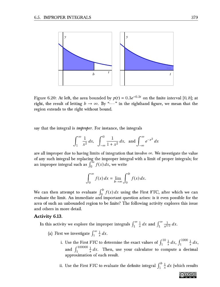
Figure 6.20: At left, the area bounded by p(t) = 0.3e −0.3t on the finite interval [0, b]; at
right, the result of letting b → ∞. By “· · · ” in the righthand figure, we mean that the
region extends to the right without bound.
say that the integral is improper. For instance, the integrals
∞
1
1
x 2 dx,
0
−∞
1
1 + x 2 dx, and
∞
−∞
e
−x 2 dx
are all improper due to having limits of integration that involve ∞. We investigate the value
of any such integral be replacing the improper integral with a limit of proper integrals; for
an improper integral such as
∞
0
f (x) dx, we write
∞
0
f (x) dx = lim
b→∞
b
0
f (x) dx.
We can then attempt to evaluate
b
0
f (x) dx using the First FTC, after which we can
evaluate the limit. An immediate and important question arises: is it even possible for the
area of such an unbounded region to be finite? The following activity explores this issue
and others in more detail.
Activity 6.13.
In this activity we explore the improper integrals
∞
1
1
x dx and
∞
1
1
x 3/2 dx.
(a) First we investigate
∞
1
1
x dx.
i. Use the First FTC to determine the exact values of
10
1
1
x dx,
1000
1
1
x dx,
and
100000
1
1
x dx. Then, use your calculator to compute a decimal
approximation of each result.
ii. Use the First FTC to evaluate the definite integral
b
1
1
x dx (which results
379
y
t
b
y
t
· · ·
Figure 6.20: At left, the area bounded by p(t) = 0.3e −0.3t on the finite interval [0, b]; at
right, the result of letting b → ∞. By “· · · ” in the righthand figure, we mean that the
region extends to the right without bound.
say that the integral is improper. For instance, the integrals
∞
1
1
x 2 dx,
0
−∞
1
1 + x 2 dx, and
∞
−∞
e
−x 2 dx
are all improper due to having limits of integration that involve ∞. We investigate the value
of any such integral be replacing the improper integral with a limit of proper integrals; for
an improper integral such as
∞
0
f (x) dx, we write
∞
0
f (x) dx = lim
b→∞
b
0
f (x) dx.
We can then attempt to evaluate
b
0
f (x) dx using the First FTC, after which we can
evaluate the limit. An immediate and important question arises: is it even possible for the
area of such an unbounded region to be finite? The following activity explores this issue
and others in more detail.
Activity 6.13.
In this activity we explore the improper integrals
∞
1
1
x dx and
∞
1
1
x 3/2 dx.
(a) First we investigate
∞
1
1
x dx.
i. Use the First FTC to determine the exact values of
10
1
1
x dx,
1000
1
1
x dx,
and
100000
1
1
x dx. Then, use your calculator to compute a decimal
approximation of each result.
ii. Use the First FTC to evaluate the definite integral
b
1
1
x dx (which results