

322
5.6. NUMERICAL INTEGRATION
y = f (x)
x 0
x 1
x 2
x 3
D 1
D 2
D 3
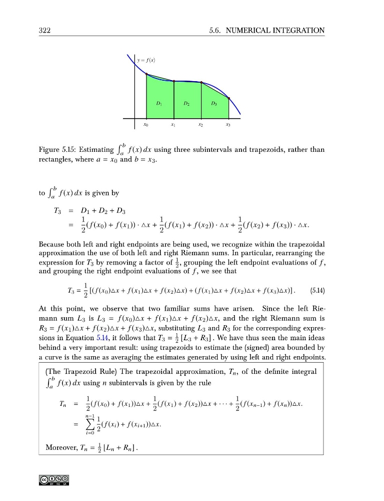
Figure 5.15: Estimating
b
a
f (x) dx using three subintervals and trapezoids, rather than
rectangles, where a = x 0 and b = x 3 .
to
b
a
f (x) dx is given by
T 3 = D 1 + D 2 + D 3
=
1
2
( f (x 0 ) + f (x 1 )) · △x +
1
2
( f (x 1 ) + f (x 2 )) · △x +
1
2
( f (x 2 ) + f (x 3 )) · △x.
Because both left and right endpoints are being used, we recognize within the trapezoidal
approximation the use of both left and right Riemann sums. In particular, rearranging the
expression for T 3 by removing a factor of
1
2 , grouping the left endpoint evaluations of f ,
and grouping the right endpoint evaluations of f , we see that
T 3 =
1
2
[( f (x 0 )△x + f (x 1 )△x + f (x 2 )△x) + ( f (x 1 )△x + f (x 2 )△x + f (x 3 )△x)] .
(5.14)
At this point, we observe that two familiar sums have arisen. Since the left Riemann sum L 3 is L 3 = f (x 0 )△x + f (x 1 )△x + f (x 2 )△x, and the right Riemann sum is
R 3 = f (x 1 )△x + f (x 2 )△x + f (x 3 )△x, substituting L 3 and R 3 for the corresponding expressions in Equation 5.14, it follows that T 3 =
1
2 [L 3 + R 3 ] . We have thus seen the main ideas
behind a very important result: using trapezoids to estimate the (signed) area bounded by
a curve is the same as averaging the estimates generated by using left and right endpoints.
(The Trapezoid Rule) The trapezoidal approximation, T n , of the definite integral
b
a
f (x) dx using n subintervals is given by the rule
T n =
1
2
( f (x 0 ) + f (x 1 ))△x +
1
2
( f (x 1 ) + f (x 2 ))△x + · · · +
1
2
( f (x n−1 ) + f (x n ))△x.
=
n−1
i=0
1
2
( f (x i ) + f (x i+1 ))△x.
Moreover, T n =
1
2 [L n + R n ] .
5.6. NUMERICAL INTEGRATION
y = f (x)
x 0
x 1
x 2
x 3
D 1
D 2
D 3
Figure 5.15: Estimating
b
a
f (x) dx using three subintervals and trapezoids, rather than
rectangles, where a = x 0 and b = x 3 .
to
b
a
f (x) dx is given by
T 3 = D 1 + D 2 + D 3
=
1
2
( f (x 0 ) + f (x 1 )) · △x +
1
2
( f (x 1 ) + f (x 2 )) · △x +
1
2
( f (x 2 ) + f (x 3 )) · △x.
Because both left and right endpoints are being used, we recognize within the trapezoidal
approximation the use of both left and right Riemann sums. In particular, rearranging the
expression for T 3 by removing a factor of
1
2 , grouping the left endpoint evaluations of f ,
and grouping the right endpoint evaluations of f , we see that
T 3 =
1
2
[( f (x 0 )△x + f (x 1 )△x + f (x 2 )△x) + ( f (x 1 )△x + f (x 2 )△x + f (x 3 )△x)] .
(5.14)
At this point, we observe that two familiar sums have arisen. Since the left Riemann sum L 3 is L 3 = f (x 0 )△x + f (x 1 )△x + f (x 2 )△x, and the right Riemann sum is
R 3 = f (x 1 )△x + f (x 2 )△x + f (x 3 )△x, substituting L 3 and R 3 for the corresponding expressions in Equation 5.14, it follows that T 3 =
1
2 [L 3 + R 3 ] . We have thus seen the main ideas
behind a very important result: using trapezoids to estimate the (signed) area bounded by
a curve is the same as averaging the estimates generated by using left and right endpoints.
(The Trapezoid Rule) The trapezoidal approximation, T n , of the definite integral
b
a
f (x) dx using n subintervals is given by the rule
T n =
1
2
( f (x 0 ) + f (x 1 ))△x +
1
2
( f (x 1 ) + f (x 2 ))△x + · · · +
1
2
( f (x n−1 ) + f (x n ))△x.
=
n−1
i=0
1
2
( f (x i ) + f (x i+1 ))△x.
Moreover, T n =
1
2 [L n + R n ] .