

320
5.6. NUMERICAL INTEGRATION
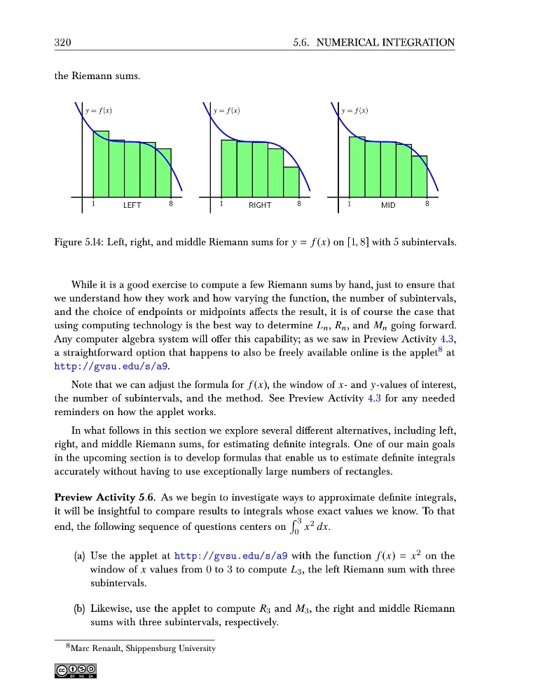
the Riemann sums.
1
8
y = f (x)
LEFT
1
8
y = f (x)
RIGHT
1
8
y = f (x)
MID
Figure 5.14: Left, right, and middle Riemann sums for y = f (x) on [1, 8] with 5 subintervals.
While it is a good exercise to compute a few Riemann sums by hand, just to ensure that
we understand how they work and how varying the function, the number of subintervals,
and the choice of endpoints or midpoints affects the result, it is of course the case that
using computing technology is the best way to determine L n , R n , and M n going forward.
Any computer algebra system will offer this capability; as we saw in Preview Activity 4.3,
a straightforward option that happens to also be freely available online is the applet 8 at
http://gvsu.edu/s/a9.
Note that we can adjust the formula for f (x), the window of x- and y-values of interest,
the number of subintervals, and the method. See Preview Activity 4.3 for any needed
reminders on how the applet works.
In what follows in this section we explore several different alternatives, including left,
right, and middle Riemann sums, for estimating definite integrals. One of our main goals
in the upcoming section is to develop formulas that enable us to estimate definite integrals
accurately without having to use exceptionally large numbers of rectangles.
Preview Activity 5.6. As we begin to investigate ways to approximate definite integrals,
it will be insightful to compare results to integrals whose exact values we know. To that
end, the following sequence of questions centers on
3
0
x 2 dx.
(a) Use the applet at http://gvsu.edu/s/a9 with the function f (x) = x 2 on the
window of x values from 0 to 3 to compute L 3 , the left Riemann sum with three
subintervals.
(b) Likewise, use the applet to compute R 3 and M 3 , the right and middle Riemann
sums with three subintervals, respectively.
8 Marc Renault, Shippensburg University
5.6. NUMERICAL INTEGRATION
the Riemann sums.
1
8
y = f (x)
LEFT
1
8
y = f (x)
RIGHT
1
8
y = f (x)
MID
Figure 5.14: Left, right, and middle Riemann sums for y = f (x) on [1, 8] with 5 subintervals.
While it is a good exercise to compute a few Riemann sums by hand, just to ensure that
we understand how they work and how varying the function, the number of subintervals,
and the choice of endpoints or midpoints affects the result, it is of course the case that
using computing technology is the best way to determine L n , R n , and M n going forward.
Any computer algebra system will offer this capability; as we saw in Preview Activity 4.3,
a straightforward option that happens to also be freely available online is the applet 8 at
http://gvsu.edu/s/a9.
Note that we can adjust the formula for f (x), the window of x- and y-values of interest,
the number of subintervals, and the method. See Preview Activity 4.3 for any needed
reminders on how the applet works.
In what follows in this section we explore several different alternatives, including left,
right, and middle Riemann sums, for estimating definite integrals. One of our main goals
in the upcoming section is to develop formulas that enable us to estimate definite integrals
accurately without having to use exceptionally large numbers of rectangles.
Preview Activity 5.6. As we begin to investigate ways to approximate definite integrals,
it will be insightful to compare results to integrals whose exact values we know. To that
end, the following sequence of questions centers on
3
0
x 2 dx.
(a) Use the applet at http://gvsu.edu/s/a9 with the function f (x) = x 2 on the
window of x values from 0 to 3 to compute L 3 , the left Riemann sum with three
subintervals.
(b) Likewise, use the applet to compute R 3 and M 3 , the right and middle Riemann
sums with three subintervals, respectively.
8 Marc Renault, Shippensburg University