

282
5.2. THE SECOND FUNDAMENTAL THEOREM OF CALCULUS
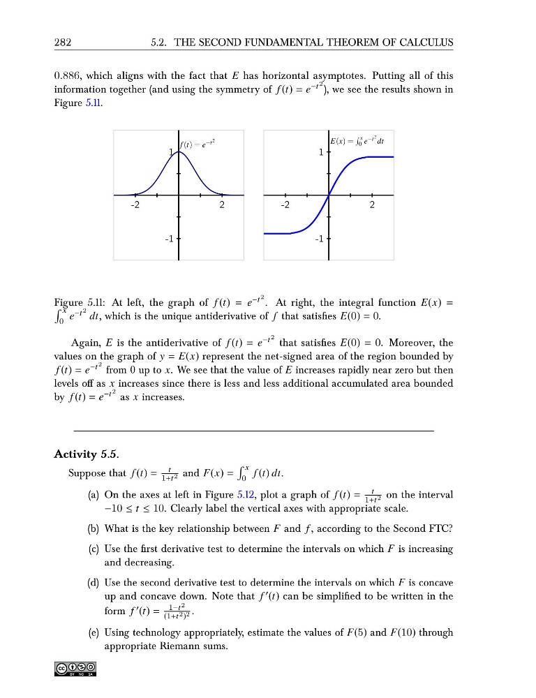
0.886, which aligns with the fact that E has horizontal asymptotes. Putting all of this
information together (and using the symmetry of f (t) = e −t 2 ), we see the results shown in
Figure 5.11.
-1
1
-2
2
f (t) = e −t 2
-1
1
-2
2
E(x) =
x
0 e −t 2 dt
Figure 5.11: At left, the graph of f (t) = e −t 2 . At right, the integral function E(x) =
x
0
e −t 2 dt, which is the unique antiderivative of f that satisfies E(0) = 0.
Again, E is the antiderivative of f (t) = e −t 2 that satisfies E(0) = 0. Moreover, the
values on the graph of y = E(x) represent the net-signed area of the region bounded by
f (t) = e −t 2 from 0 up to x. We see that the value of E increases rapidly near zero but then
levels off as x increases since there is less and less additional accumulated area bounded
by f (t) = e −t 2 as x increases.
Activity 5.5.
Suppose that f (t) =
t
1+t 2 and F(x) =
x
0
f (t) dt.
(a) On the axes at left in Figure 5.12, plot a graph of f (t) =
t
1+t 2 on the interval
−10 ≤ t ≤ 10. Clearly label the vertical axes with appropriate scale.
(b) What is the key relationship between F and f , according to the Second FTC?
(c) Use the first derivative test to determine the intervals on which F is increasing
and decreasing.
(d) Use the second derivative test to determine the intervals on which F is concave
up and concave down. Note that f ′ (t) can be simplified to be written in the
form f ′ (t) =
1−t 2
(1+t 2 ) 2 .
(e) Using technology appropriately, estimate the values of F(5) and F(10) through
appropriate Riemann sums.
5.2. THE SECOND FUNDAMENTAL THEOREM OF CALCULUS
0.886, which aligns with the fact that E has horizontal asymptotes. Putting all of this
information together (and using the symmetry of f (t) = e −t 2 ), we see the results shown in
Figure 5.11.
-1
1
-2
2
f (t) = e −t 2
-1
1
-2
2
E(x) =
x
0 e −t 2 dt
Figure 5.11: At left, the graph of f (t) = e −t 2 . At right, the integral function E(x) =
x
0
e −t 2 dt, which is the unique antiderivative of f that satisfies E(0) = 0.
Again, E is the antiderivative of f (t) = e −t 2 that satisfies E(0) = 0. Moreover, the
values on the graph of y = E(x) represent the net-signed area of the region bounded by
f (t) = e −t 2 from 0 up to x. We see that the value of E increases rapidly near zero but then
levels off as x increases since there is less and less additional accumulated area bounded
by f (t) = e −t 2 as x increases.
Activity 5.5.
Suppose that f (t) =
t
1+t 2 and F(x) =
x
0
f (t) dt.
(a) On the axes at left in Figure 5.12, plot a graph of f (t) =
t
1+t 2 on the interval
−10 ≤ t ≤ 10. Clearly label the vertical axes with appropriate scale.
(b) What is the key relationship between F and f , according to the Second FTC?
(c) Use the first derivative test to determine the intervals on which F is increasing
and decreasing.
(d) Use the second derivative test to determine the intervals on which F is concave
up and concave down. Note that f ′ (t) can be simplified to be written in the
form f ′ (t) =
1−t 2
(1+t 2 ) 2 .
(e) Using technology appropriately, estimate the values of F(5) and F(10) through
appropriate Riemann sums.