

280
5.2. THE SECOND FUNDAMENTAL THEOREM OF CALCULUS
1
2
3
4
5
6
7
-1
1
y = f (x)
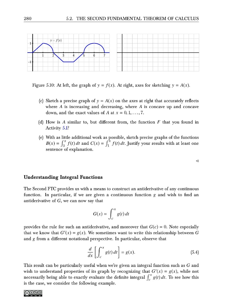
Figure 5.10: At left, the graph of y = f (x). At right, axes for sketching y = A(x).
(c) Sketch a precise graph of y = A(x) on the axes at right that accurately reflects
where A is increasing and decreasing, where A is concave up and concave
down, and the exact values of A at x = 0, 1, . . . , 7.
(d) How is A similar to, but different from, the function F that you found in
Activity 5.1?
(e) With as little additional work as possible, sketch precise graphs of the functions
B(x) =
x
3
f (t) dt and C(x) =
x
1
f (t) dt. Justify your results with at least one
sentence of explanation.
⊳
Understanding Integral Functions
The Second FTC provides us with a means to construct an antiderivative of any continuous
function. In particular, if we are given a continuous function g and wish to find an
antiderivative of G, we can now say that
G(x) =
x
c
g(t) dt
provides the rule for such an antiderivative, and moreover that G(c) = 0. Note especially
that we know that G ′ (x) = g(x). We sometimes want to write this relationship between G
and g from a different notational perspective. In particular, observe that
d
dx
x
c
g(t) dt
= g(x).
(5.4)
This result can be particularly useful when we’re given an integral function such as G and
wish to understand properties of its graph by recognizing that G ′ (x) = g(x), while not
necessarily being able to exactly evaluate the definite integral
x
c
g(t) dt. To see how this
is the case, we consider the following example.
5.2. THE SECOND FUNDAMENTAL THEOREM OF CALCULUS
1
2
3
4
5
6
7
-1
1
y = f (x)
Figure 5.10: At left, the graph of y = f (x). At right, axes for sketching y = A(x).
(c) Sketch a precise graph of y = A(x) on the axes at right that accurately reflects
where A is increasing and decreasing, where A is concave up and concave
down, and the exact values of A at x = 0, 1, . . . , 7.
(d) How is A similar to, but different from, the function F that you found in
Activity 5.1?
(e) With as little additional work as possible, sketch precise graphs of the functions
B(x) =
x
3
f (t) dt and C(x) =
x
1
f (t) dt. Justify your results with at least one
sentence of explanation.
⊳
Understanding Integral Functions
The Second FTC provides us with a means to construct an antiderivative of any continuous
function. In particular, if we are given a continuous function g and wish to find an
antiderivative of G, we can now say that
G(x) =
x
c
g(t) dt
provides the rule for such an antiderivative, and moreover that G(c) = 0. Note especially
that we know that G ′ (x) = g(x). We sometimes want to write this relationship between G
and g from a different notational perspective. In particular, observe that
d
dx
x
c
g(t) dt
= g(x).
(5.4)
This result can be particularly useful when we’re given an integral function such as G and
wish to understand properties of its graph by recognizing that G ′ (x) = g(x), while not
necessarily being able to exactly evaluate the definite integral
x
c
g(t) dt. To see how this
is the case, we consider the following example.