

272
5.1. CONSTRUCTING ACCURATE GRAPHS OF ANTIDERIVATIVES
-1
1
y = f (t)
π
2π
x
1
3
π
2π
x
A(x)
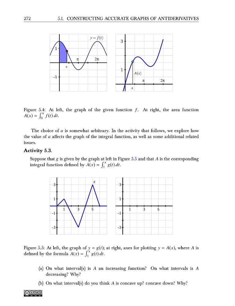
Figure 5.4: At left, the graph of the given function f . At right, the area function
A(x) =
x
0
f (t) dt.
The choice of a is somewhat arbitrary. In the activity that follows, we explore how
the value of a affects the graph of the integral function, as well as some additional related
issues.
Activity 5.3.
Suppose that g is given by the graph at left in Figure 5.5 and that A is the corresponding
integral function defined by A(x) =
x
1
g(t) dt.
1
3
5
-3
-1
1
3
g
1
3
5
-3
-1
1
3
Figure 5.5: At left, the graph of y = g(t); at right, axes for plotting y = A(x), where A is
defined by the formula A(x) =
x
1
g(t) dt.
(a) On what interval(s) is A an increasing function? On what intervals is A
decreasing? Why?
(b) On what interval(s) do you think A is concave up? concave down? Why?
5.1. CONSTRUCTING ACCURATE GRAPHS OF ANTIDERIVATIVES
-1
1
y = f (t)
π
2π
x
1
3
π
2π
x
A(x)
Figure 5.4: At left, the graph of the given function f . At right, the area function
A(x) =
x
0
f (t) dt.
The choice of a is somewhat arbitrary. In the activity that follows, we explore how
the value of a affects the graph of the integral function, as well as some additional related
issues.
Activity 5.3.
Suppose that g is given by the graph at left in Figure 5.5 and that A is the corresponding
integral function defined by A(x) =
x
1
g(t) dt.
1
3
5
-3
-1
1
3
g
1
3
5
-3
-1
1
3
Figure 5.5: At left, the graph of y = g(t); at right, axes for plotting y = A(x), where A is
defined by the formula A(x) =
x
1
g(t) dt.
(a) On what interval(s) is A an increasing function? On what intervals is A
decreasing? Why?
(b) On what interval(s) do you think A is concave up? concave down? Why?