

156
2.8. USING DERIVATIVES TO EVALUATE LIMITS
the logarithm function does. We’ll soon use limits to quantify what we mean by “quickly.”
-4
4
8
-4
4
8
y = e x
y = ln(x)
-2
2
-64
64
y = f (x)
y = g(x)
10
1
y = sin(x)
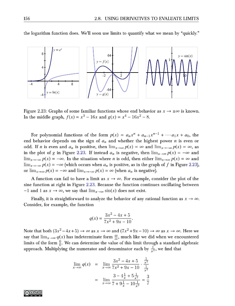
Figure 2.23: Graphs of some familiar functions whose end behavior as x → ±∞ is known.
In the middle graph, f (x) = x 3 − 16x and g(x) = x 4 − 16x 2 − 8.
For polynomial functions of the form p(x) = a n x n + a n−1 x n−1 + · · · a 1 x + a 0 , the
end behavior depends on the sign of a n and whether the highest power n is even or
odd. If n is even and a n is positive, then lim x→∞ p(x) = ∞ and lim x→−∞ p(x) = ∞, as
in the plot of g in Figure 2.23. If instead a n is negative, then lim x→∞ p(x) = −∞ and
lim x→−∞ p(x) = −∞. In the situation where n is odd, then either lim x→∞ p(x) = ∞ and
lim x→−∞ p(x) = −∞ (which occurs when a n is positive, as in the graph of f in Figure 2.23),
or lim x→∞ p(x) = −∞ and lim x→−∞ p(x) = ∞ (when a n is negative).
A function can fail to have a limit as x → ∞. For example, consider the plot of the
sine function at right in Figure 2.23. Because the function continues oscillating between
−1 and 1 as x → ∞, we say that lim x→∞ sin(x) does not exist.
Finally, it is straightforward to analyze the behavior of any rational function as x → ∞.
Consider, for example, the function
q(x) =
3x 2 − 4x + 5
7x 2 + 9x − 10
.
Note that both (3x 2 − 4x + 5) → ∞ as x → ∞ and (7x 2 + 9x − 10) → ∞ as x → ∞. Here we
say that lim x→∞ q(x) has indeterminate form
∞
∞ , much like we did when we encountered
limits of the form
0
0 . We can determine the value of this limit through a standard algebraic
approach. Multiplying the numerator and denominator each by
1
x 2 , we find that
lim
x→∞
q(x) = lim
x→∞
3x 2 − 4x + 5
7x 2 + 9x − 10
·
1
x 2
1
x 2
= lim
x→∞
3 − 4
1
x + 5
1
x 2
7 + 9
1
x − 10
1
x 2
=
3
7
2.8. USING DERIVATIVES TO EVALUATE LIMITS
the logarithm function does. We’ll soon use limits to quantify what we mean by “quickly.”
-4
4
8
-4
4
8
y = e x
y = ln(x)
-2
2
-64
64
y = f (x)
y = g(x)
10
1
y = sin(x)
Figure 2.23: Graphs of some familiar functions whose end behavior as x → ±∞ is known.
In the middle graph, f (x) = x 3 − 16x and g(x) = x 4 − 16x 2 − 8.
For polynomial functions of the form p(x) = a n x n + a n−1 x n−1 + · · · a 1 x + a 0 , the
end behavior depends on the sign of a n and whether the highest power n is even or
odd. If n is even and a n is positive, then lim x→∞ p(x) = ∞ and lim x→−∞ p(x) = ∞, as
in the plot of g in Figure 2.23. If instead a n is negative, then lim x→∞ p(x) = −∞ and
lim x→−∞ p(x) = −∞. In the situation where n is odd, then either lim x→∞ p(x) = ∞ and
lim x→−∞ p(x) = −∞ (which occurs when a n is positive, as in the graph of f in Figure 2.23),
or lim x→∞ p(x) = −∞ and lim x→−∞ p(x) = ∞ (when a n is negative).
A function can fail to have a limit as x → ∞. For example, consider the plot of the
sine function at right in Figure 2.23. Because the function continues oscillating between
−1 and 1 as x → ∞, we say that lim x→∞ sin(x) does not exist.
Finally, it is straightforward to analyze the behavior of any rational function as x → ∞.
Consider, for example, the function
q(x) =
3x 2 − 4x + 5
7x 2 + 9x − 10
.
Note that both (3x 2 − 4x + 5) → ∞ as x → ∞ and (7x 2 + 9x − 10) → ∞ as x → ∞. Here we
say that lim x→∞ q(x) has indeterminate form
∞
∞ , much like we did when we encountered
limits of the form
0
0 . We can determine the value of this limit through a standard algebraic
approach. Multiplying the numerator and denominator each by
1
x 2 , we find that
lim
x→∞
q(x) = lim
x→∞
3x 2 − 4x + 5
7x 2 + 9x − 10
·
1
x 2
1
x 2
= lim
x→∞
3 − 4
1
x + 5
1
x 2
7 + 9
1
x − 10
1
x 2
=
3
7