

154
2.8. USING DERIVATIVES TO EVALUATE LIMITS
value of
lim
x→2
p(x)
q(x)
.
(c) Use the right-hand graph to compute r(2), r ′ (2), s(2), s ′ (2). Explain why you
cannot determine the exact value of
lim
x→2
r(x)
s(x)
without further information being provided, but that you can determine the
sign of lim x→2
r(x)
s(x) . In addition, state what the sign of the limit will be, with
justification.
⊳
Limits involving ∞
The concept of infinity, denoted ∞, arises naturally in calculus, like it does in much of
mathematics. It is important to note from the outset that ∞ is a concept, but not a number
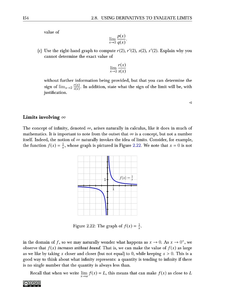
itself. Indeed, the notion of ∞ naturally invokes the idea of limits. Consider, for example,
the function f (x) =
1
x , whose graph is pictured in Figure 2.22. We note that x = 0 is not
1
1
f (x) =
1
x
Figure 2.22: The graph of f (x) =
1
x .
in the domain of f , so we may naturally wonder what happens as x → 0. As x → 0 + , we
observe that f (x) increases without bound. That is, we can make the value of f (x) as large
as we like by taking x closer and closer (but not equal) to 0, while keeping x > 0. This is a
good way to think about what infinity represents: a quantity is tending to infinity if there
is no single number that the quantity is always less than.
Recall that when we write lim
x→a
f (x) = L, this means that can make f (x) as close to L
2.8. USING DERIVATIVES TO EVALUATE LIMITS
value of
lim
x→2
p(x)
q(x)
.
(c) Use the right-hand graph to compute r(2), r ′ (2), s(2), s ′ (2). Explain why you
cannot determine the exact value of
lim
x→2
r(x)
s(x)
without further information being provided, but that you can determine the
sign of lim x→2
r(x)
s(x) . In addition, state what the sign of the limit will be, with
justification.
⊳
Limits involving ∞
The concept of infinity, denoted ∞, arises naturally in calculus, like it does in much of
mathematics. It is important to note from the outset that ∞ is a concept, but not a number
itself. Indeed, the notion of ∞ naturally invokes the idea of limits. Consider, for example,
the function f (x) =
1
x , whose graph is pictured in Figure 2.22. We note that x = 0 is not
1
1
f (x) =
1
x
Figure 2.22: The graph of f (x) =
1
x .
in the domain of f , so we may naturally wonder what happens as x → 0. As x → 0 + , we
observe that f (x) increases without bound. That is, we can make the value of f (x) as large
as we like by taking x closer and closer (but not equal) to 0, while keeping x > 0. This is a
good way to think about what infinity represents: a quantity is tending to infinity if there
is no single number that the quantity is always less than.
Recall that when we write lim
x→a
f (x) = L, this means that can make f (x) as close to L