

150
2.8. USING DERIVATIVES TO EVALUATE LIMITS
(c) Next we will investigate the behavior of both the numerator and denominator of h
near the point where x = 1. Let f (x) = x 5 + x − 2 and g(x) = x 2 − 1. Find the
local linearizations of f and g at a = 1, and call these functions L f (x) and L g (x),
respectively.
(d) Explain why h(x) ≈
L f (x)
L g (x)
for x near a = 1.
(e) Using your work from (c) and (d), evaluate
lim
x→1
L f (x)
L g (x)
.
What do you think your result tells us about lim
x→1
h(x)?
(f) Investigate the function h(x) graphically and numerically near x = 1. What do
you think is the value of lim
x→1
h(x)?
⊲⊳
Using derivatives to evaluate indeterminate limits of the form
0
0 .
a
g
L g
f
L f
a
L g ≈ g
L f ≈ f
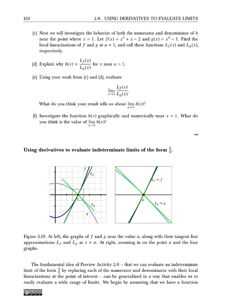
Figure 2.19: At left, the graphs of f and g near the value a, along with their tangent line
approximations L f and L g at x = a. At right, zooming in on the point a and the four
graphs.
The fundamental idea of Preview Activity 2.8 – that we can evaluate an indeterminate
limit of the form
0
0 by replacing each of the numerator and denominator with their local
linearizations at the point of interest – can be generalized in a way that enables us to
easily evaluate a wide range of limits. We begin by assuming that we have a function
2.8. USING DERIVATIVES TO EVALUATE LIMITS
(c) Next we will investigate the behavior of both the numerator and denominator of h
near the point where x = 1. Let f (x) = x 5 + x − 2 and g(x) = x 2 − 1. Find the
local linearizations of f and g at a = 1, and call these functions L f (x) and L g (x),
respectively.
(d) Explain why h(x) ≈
L f (x)
L g (x)
for x near a = 1.
(e) Using your work from (c) and (d), evaluate
lim
x→1
L f (x)
L g (x)
.
What do you think your result tells us about lim
x→1
h(x)?
(f) Investigate the function h(x) graphically and numerically near x = 1. What do
you think is the value of lim
x→1
h(x)?
⊲⊳
Using derivatives to evaluate indeterminate limits of the form
0
0 .
a
g
L g
f
L f
a
L g ≈ g
L f ≈ f
Figure 2.19: At left, the graphs of f and g near the value a, along with their tangent line
approximations L f and L g at x = a. At right, zooming in on the point a and the four
graphs.
The fundamental idea of Preview Activity 2.8 – that we can evaluate an indeterminate
limit of the form
0
0 by replacing each of the numerator and denominator with their local
linearizations at the point of interest – can be generalized in a way that enables us to
easily evaluate a wide range of limits. We begin by assuming that we have a function