

2.6. DERIVATIVES OF INVERSE FUNCTIONS
133
-4
4
8
-4
4
8
y = e x
y = ln(x)
A
B
A ′
B ′
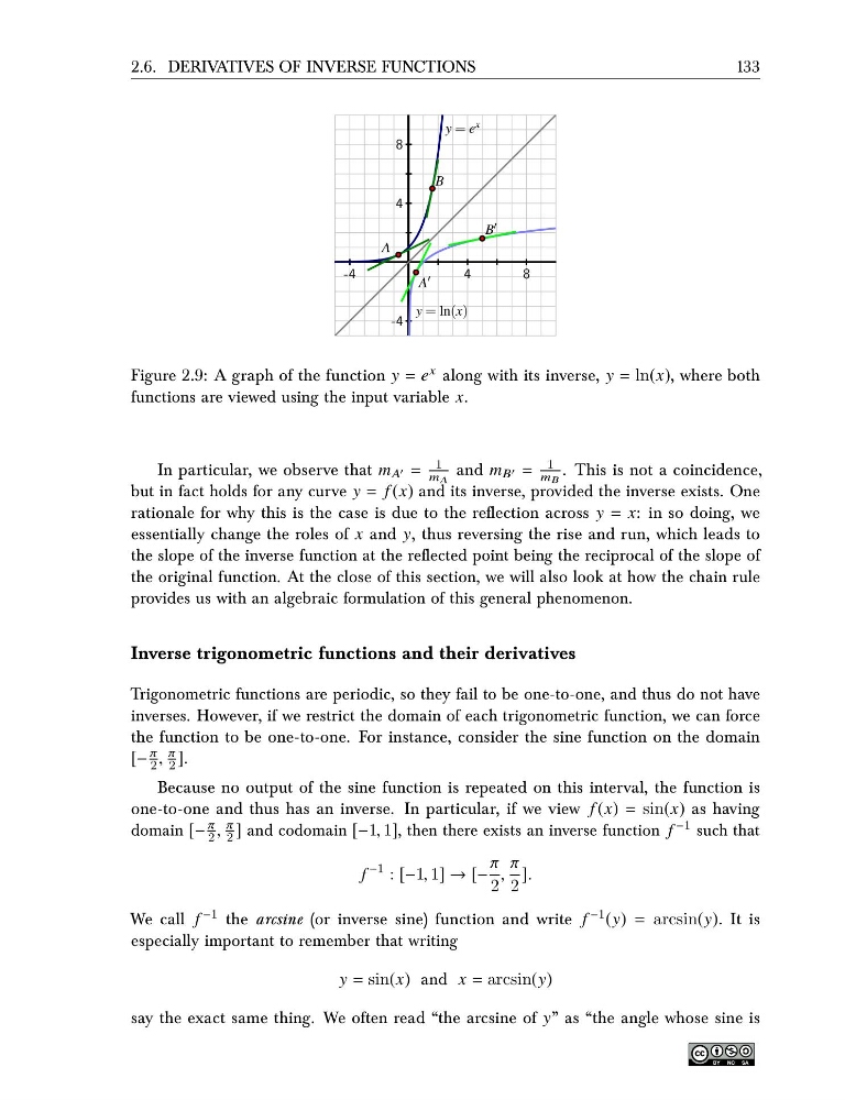
Figure 2.9: A graph of the function y = e x along with its inverse, y = ln(x), where both
functions are viewed using the input variable x.
In particular, we observe that m A ′ =
1
m A
and m B ′ =
1
m B
. This is not a coincidence,
but in fact holds for any curve y = f (x) and its inverse, provided the inverse exists. One
rationale for why this is the case is due to the reflection across y = x: in so doing, we
essentially change the roles of x and y, thus reversing the rise and run, which leads to
the slope of the inverse function at the reflected point being the reciprocal of the slope of
the original function. At the close of this section, we will also look at how the chain rule
provides us with an algebraic formulation of this general phenomenon.
Inverse trigonometric functions and their derivatives
Trigonometric functions are periodic, so they fail to be one-to-one, and thus do not have
inverses. However, if we restrict the domain of each trigonometric function, we can force
the function to be one-to-one. For instance, consider the sine function on the domain
[−
π
2 ,
π
2 ].
Because no output of the sine function is repeated on this interval, the function is
one-to-one and thus has an inverse. In particular, if we view f (x) = sin(x) as having
domain [−
π
2 ,
π
2 ] and codomain [−1, 1], then there exists an inverse function f −1 such that
f
−1 : [−1, 1] → [−
π
2
,
π
2
].
We call f −1 the arcsine (or inverse sine) function and write f −1 (y) = arcsin(y). It is
especially important to remember that writing
y = sin(x) and x = arcsin(y)
say the exact same thing. We often read “the arcsine of y” as “the angle whose sine is
133
-4
4
8
-4
4
8
y = e x
y = ln(x)
A
B
A ′
B ′
Figure 2.9: A graph of the function y = e x along with its inverse, y = ln(x), where both
functions are viewed using the input variable x.
In particular, we observe that m A ′ =
1
m A
and m B ′ =
1
m B
. This is not a coincidence,
but in fact holds for any curve y = f (x) and its inverse, provided the inverse exists. One
rationale for why this is the case is due to the reflection across y = x: in so doing, we
essentially change the roles of x and y, thus reversing the rise and run, which leads to
the slope of the inverse function at the reflected point being the reciprocal of the slope of
the original function. At the close of this section, we will also look at how the chain rule
provides us with an algebraic formulation of this general phenomenon.
Inverse trigonometric functions and their derivatives
Trigonometric functions are periodic, so they fail to be one-to-one, and thus do not have
inverses. However, if we restrict the domain of each trigonometric function, we can force
the function to be one-to-one. For instance, consider the sine function on the domain
[−
π
2 ,
π
2 ].
Because no output of the sine function is repeated on this interval, the function is
one-to-one and thus has an inverse. In particular, if we view f (x) = sin(x) as having
domain [−
π
2 ,
π
2 ] and codomain [−1, 1], then there exists an inverse function f −1 such that
f
−1 : [−1, 1] → [−
π
2
,
π
2
].
We call f −1 the arcsine (or inverse sine) function and write f −1 (y) = arcsin(y). It is
especially important to remember that writing
y = sin(x) and x = arcsin(y)
say the exact same thing. We often read “the arcsine of y” as “the angle whose sine is