THE STRONG COUPLING EXPANSION
41
complicated gauge groups, like 0(2) or SU(N) the sm allexpansion is
similar with the only difference that the plaquettes carry conserved
quantum numbers just as it was in the case of paths, describing systems
with global symmetries.
We see that there exists a very general rule that the strong coupling
expansion for a gauge system is obtained from the corresponding global
system by replacing paths by surfaces. The physical meaning of this rule
becomes transparent in the Hamiltonian language. Let us pass to the
hamiltonian in the 0(2) case (other cases are similar). As before, to do
this we introduce anisotropy in the “time” direction into the formula
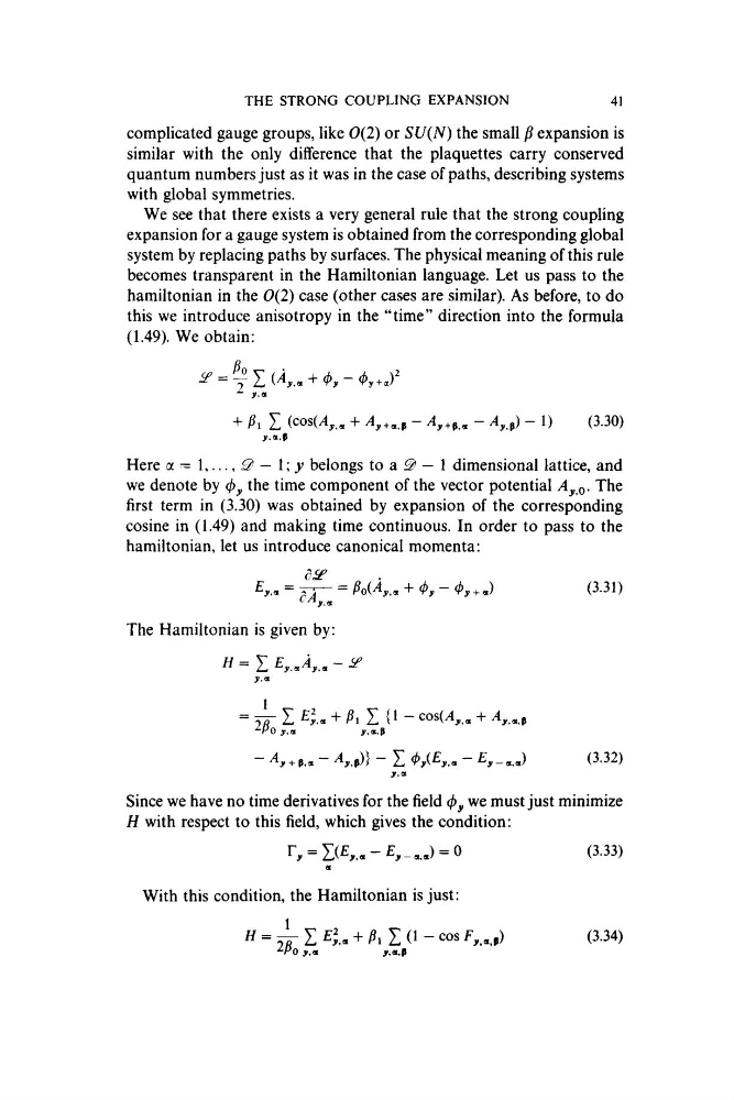
(1.49). We obtain:
^ = y I
+ y
+ ^1 Z
+
+
“ 1)
(3.30)
Here a — 1 , . . . , ^ — I, y belongs to a ^ — 1 dimensional lattice, and
we denote by (py the time component of the vector potential Ay ^. The
first term in (3.30) was obtained by expansion of the corresponding
cosine in (1.49) and making time continuous. In order to pass to the
hamiltonian, let us introduce canonical momenta:
dA^ —
+ 4 > y — < P y + ,)
(3.31)
The Hamiltonian is given by:
« = I
y < 3 i
1
yy Z
Z {1 - cos(T,., +
y . t t
y . « . p
(3.32)
Since we have no time derivatives for the field (py we must just minimize
H with respect to this field, which gives the condition:
r . = Z(£..,= 0
(3.33)
With this condition, the Hamiltonian is just:
W = i Z £ L + ^ Z O -c o s T ,...,)
^Po y,a
J,« ,p
(3.34)