

3.1 Ising Model
34
GAUGE FIELDS AND STRINGS
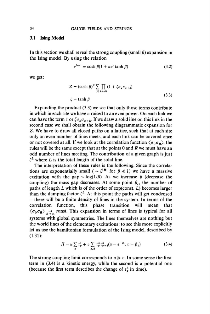
In this section we shall reveal the strong coupling (small j?) expansion in
the Ising model. By using the relation
(3.2)
we get:
z = {coshßrY.
+
{
(3.3)
Expanding the product (3.3) we see that only those terms contribute
in which in each site we have a raised to an even power. On each link we
can have the term 1 or
If we draw a solid line on this link in the
second case we shall obtain the following diagrammatic expansion for
Z. We have to draw all closed paths on a lattice, such that at each site
only an even number of lines meets, and each link can be covered once
or not covered at all. If we look at the correlation function
the
rules will be the same except that at the points 0 and R we must have an
odd number of lines meeting. The contribution of a given graph is just
where L is the total length of the solid line.
The interpretation of these rules is the following. Since the correlations are exponentially small ( ^
for
1) we have a massive
excitation with the gap ^ log(l/j5). As we increase p (decrease the
coupling) the mass gap decreases. At some point
the number of
paths of length L which is of the order of exp(const. L) becomes larger
than the damping factor C^. At this point the paths will get condensed
—there will be a finite density of lines in the system. In terms of the
correlation function, this phase transition will mean that
const. This expansion in terms of lines is typical for all
systems with global symmetries. The lines themselves are nothing but
the world lines of the elementary excitations: to see this more explicitly
let us use the hamiltonian formulation of the Ising model, described by
(1.31):
y
(3.4)
The strong coupling limit corresponds to uP v. In some sense the first
term in (3.4) is a kinetic energy, while the second is a potential one
(because the first term describes the change of tI in time).
34
GAUGE FIELDS AND STRINGS
In this section we shall reveal the strong coupling (small j?) expansion in
the Ising model. By using the relation
(3.2)
we get:
z = {coshßrY.
+
{
(3.3)
Expanding the product (3.3) we see that only those terms contribute
in which in each site we have a raised to an even power. On each link we
can have the term 1 or
If we draw a solid line on this link in the
second case we shall obtain the following diagrammatic expansion for
Z. We have to draw all closed paths on a lattice, such that at each site
only an even number of lines meets, and each link can be covered once
or not covered at all. If we look at the correlation function
the
rules will be the same except that at the points 0 and R we must have an
odd number of lines meeting. The contribution of a given graph is just
where L is the total length of the solid line.
The interpretation of these rules is the following. Since the correlations are exponentially small ( ^
for
1) we have a massive
excitation with the gap ^ log(l/j5). As we increase p (decrease the
coupling) the mass gap decreases. At some point
the number of
paths of length L which is of the order of exp(const. L) becomes larger
than the damping factor C^. At this point the paths will get condensed
—there will be a finite density of lines in the system. In terms of the
correlation function, this phase transition will mean that
const. This expansion in terms of lines is typical for all
systems with global symmetries. The lines themselves are nothing but
the world lines of the elementary excitations: to see this more explicitly
let us use the hamiltonian formulation of the Ising model, described by
(1.31):
y
(3.4)
The strong coupling limit corresponds to uP v. In some sense the first
term in (3.4) is a kinetic energy, while the second is a potential one
(because the first term describes the change of tI in time).