

ATTEMPT AT A SYNTHESIS
285
The last form is especially interesting. It shows that we are dealing
with a Grassman (j-model, associated with the surface. The order
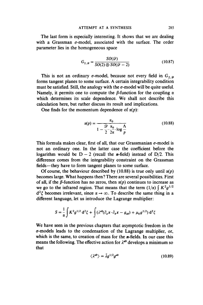
parameter lies in the homogeneous space
s o m
SO(2)®SO{^ - 2 )
(10.87)
This is not an ordinary a-model, because not every field in
forms tangent planes to some surface. A certain integrability condition
must be satisfied. Still, the analogy with the (T-model will be quite useful.
Namely, it permits one to compute the jS-function for the coupling a
which determines its scale dependence. We shall not describe this
calculation here, but rather discuss its result and implications.
One finds for the momentum dependence of a(p):
oc(p) = ■
^ ao
A
. l o g -
2 2n
p
( 10.88)
This formula makes clear, first of all, that our Grassmanian a-model is
not an ordinary one. In the latter case the coefficient before the
logarithm would be D — 2 (recall the /i-field) instead of D/2. This
difference comes from the integrability constraint on the Grassman
fields—they have to form tangent planes to some surface.
Of course, the behaviour described by (10.88) is true only until cc(p)
becomes large. What happens then? There are several possibilities. First
of all, if the j¥-function has no zeros, then oc(p) continues to increase as
we go to the infrared region. That means that the term (1/a) J
becomes irrelevant, since a -► oo. To describe the same thing in a
different language, let us introduce the Lagrange multiplier:
^ I
+ I
• df,x - g j - f
We have seen in the previous chapters that asymptotic freedom in the
(T-models leads to the condensation of the Lagrange multiplier, or,
which is the same, to creation of mass for the w-fields. In our case this
means the following. The effective action for A"*’ develops a minimum so
that
(10.89)
285
The last form is especially interesting. It shows that we are dealing
with a Grassman (j-model, associated with the surface. The order
parameter lies in the homogeneous space
s o m
SO(2)®SO{^ - 2 )
(10.87)
This is not an ordinary a-model, because not every field in
forms tangent planes to some surface. A certain integrability condition
must be satisfied. Still, the analogy with the (T-model will be quite useful.
Namely, it permits one to compute the jS-function for the coupling a
which determines its scale dependence. We shall not describe this
calculation here, but rather discuss its result and implications.
One finds for the momentum dependence of a(p):
oc(p) = ■
^ ao
A
. l o g -
2 2n
p
( 10.88)
This formula makes clear, first of all, that our Grassmanian a-model is
not an ordinary one. In the latter case the coefficient before the
logarithm would be D — 2 (recall the /i-field) instead of D/2. This
difference comes from the integrability constraint on the Grassman
fields—they have to form tangent planes to some surface.
Of course, the behaviour described by (10.88) is true only until cc(p)
becomes large. What happens then? There are several possibilities. First
of all, if the j¥-function has no zeros, then oc(p) continues to increase as
we go to the infrared region. That means that the term (1/a) J
becomes irrelevant, since a -► oo. To describe the same thing in a
different language, let us introduce the Lagrange multiplier:
^ I
+ I
• df,x - g j - f
We have seen in the previous chapters that asymptotic freedom in the
(T-models leads to the condensation of the Lagrange multiplier, or,
which is the same, to creation of mass for the w-fields. In our case this
means the following. The effective action for A"*’ develops a minimum so
that
(10.89)