

318 Basic Engineering Mathematics
5. y =
1
x
6. y = 12
7. y = x −
1
x 2
8. y = 3x 5 − 2x 4 + 5x 3 + x 2 − 1
9. y =
2
x 3
10. y = 4x(1 − x)
11. y =
√
x
12. y =
√
t 3
13. y = 6 +
1
x 3
14. y = 3x −
1
√
x
+
1
x
15. y = (x + 1) 2
16. y = x + 3
√
x
17. y = (1 − x) 2
18. y =
5
x 2 −
1
√
x 7
+ 2
19. y = 3(t − 2) 2
20. y =
(x + 2) 2
x
21. Find the gradient of the following curves at
the given points.
(a) y = 3x
2 at x = 1
(b) y =
√
x at x = 9
(c) y = x 3 + 3x − 7 at x = 0
(d) y =
1
√
x
at x = 4
(e) y =
1
x
at x = 2
(f ) y = (2x + 3)(x − 1) at x = −2
22. Differentiate f (x) = 6x 2 − 3x + 5 and find
the gradient of the curve at
(a) x = −1
(b) x = 2
23. Find the differential coefficient of
y = 2x 3 + 3x 2 − 4x − 1 and determine the
gradient of the curve at x = 2.
24. Determine the derivative of
y = −2x 3 + 4x + 7 and determine the
gradient of the curve at x = −1.5
34.6 Differentiation of sine and
cosine functions
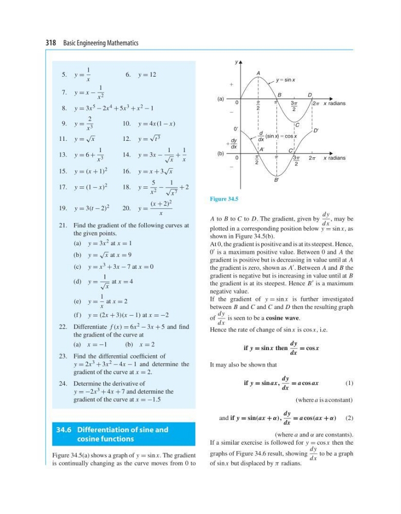
Figure 34.5(a) shows a graph of y = sin x. The gradient
is continually changing as the curve moves from 0 to
y
0
(a)
(b)
0
y 5 sin x
x radians
x radians
1
2
2
A
A9
09
C9
B9
D9
B
D
C
2
d
dx
1
dy
dx
2
2
3
2
3
2
(sin x) 5 cos x
2
Figure 34.5
A to B to C to D. The gradient, given by
dy
dx
, may be
plotted in a corresponding position below y = sin x, as
shown in Figure 34.5(b).
At 0, the gradient is positive and is at its steepest. Hence,
0 is a maximum positive value. Between 0 and A the
gradient is positive but is decreasing in value until at A
the gradient is zero, shown as A . Between A and B the
gradient is negative but is increasing in value until at B
the gradient is at its steepest. Hence B is a maximum
negative value.
If the gradient of y = sin x is further investigated
between B and C and C and D then the resulting graph
of
dy
dx
is seen to be a cosine wave.
Hence the rate of change of sin x is cos x, i.e.
if y = sin x then
dy
dx
= cos x
It may also be shown that
if y = sin ax,
dy
dx
= a cos ax
(1)
(where a is a constant)
and if y = sin(ax + α),
dy
dx
= a cos(ax + α) (2)
(where a and α are constants).
If a similar exercise is followed for y = cos x then the
graphs of Figure 34.6 result, showing
dy
dx
to be a graph
of sin x but displaced by π radians.
5. y =
1
x
6. y = 12
7. y = x −
1
x 2
8. y = 3x 5 − 2x 4 + 5x 3 + x 2 − 1
9. y =
2
x 3
10. y = 4x(1 − x)
11. y =
√
x
12. y =
√
t 3
13. y = 6 +
1
x 3
14. y = 3x −
1
√
x
+
1
x
15. y = (x + 1) 2
16. y = x + 3
√
x
17. y = (1 − x) 2
18. y =
5
x 2 −
1
√
x 7
+ 2
19. y = 3(t − 2) 2
20. y =
(x + 2) 2
x
21. Find the gradient of the following curves at
the given points.
(a) y = 3x
2 at x = 1
(b) y =
√
x at x = 9
(c) y = x 3 + 3x − 7 at x = 0
(d) y =
1
√
x
at x = 4
(e) y =
1
x
at x = 2
(f ) y = (2x + 3)(x − 1) at x = −2
22. Differentiate f (x) = 6x 2 − 3x + 5 and find
the gradient of the curve at
(a) x = −1
(b) x = 2
23. Find the differential coefficient of
y = 2x 3 + 3x 2 − 4x − 1 and determine the
gradient of the curve at x = 2.
24. Determine the derivative of
y = −2x 3 + 4x + 7 and determine the
gradient of the curve at x = −1.5
34.6 Differentiation of sine and
cosine functions
Figure 34.5(a) shows a graph of y = sin x. The gradient
is continually changing as the curve moves from 0 to
y
0
(a)
(b)
0
y 5 sin x
x radians
x radians
1
2
2
A
A9
09
C9
B9
D9
B
D
C
2
d
dx
1
dy
dx
2
2
3
2
3
2
(sin x) 5 cos x
2
Figure 34.5
A to B to C to D. The gradient, given by
dy
dx
, may be
plotted in a corresponding position below y = sin x, as
shown in Figure 34.5(b).
At 0, the gradient is positive and is at its steepest. Hence,
0 is a maximum positive value. Between 0 and A the
gradient is positive but is decreasing in value until at A
the gradient is zero, shown as A . Between A and B the
gradient is negative but is increasing in value until at B
the gradient is at its steepest. Hence B is a maximum
negative value.
If the gradient of y = sin x is further investigated
between B and C and C and D then the resulting graph
of
dy
dx
is seen to be a cosine wave.
Hence the rate of change of sin x is cos x, i.e.
if y = sin x then
dy
dx
= cos x
It may also be shown that
if y = sin ax,
dy
dx
= a cos ax
(1)
(where a is a constant)
and if y = sin(ax + α),
dy
dx
= a cos(ax + α) (2)
(where a and α are constants).
If a similar exercise is followed for y = cos x then the
graphs of Figure 34.6 result, showing
dy
dx
to be a graph
of sin x but displaced by π radians.