

Presentation of statistical data 295
Table 31.3
1
2
3
4
5
6
Class
Frequency
Upper class
Lower class
Class range
Height of
boundary
boundary
rectangle
20–40
2
45
15
30
2
30
=
1
15
50–70
6
75
45
30
6
30
=
3
15
80–90
12
95
75
20
12
20
=
9
15
100–110
14
115
95
20
14
20
=
10
1
2
15
120–140
4
145
115
30
4
30
=
2
15
150–170
2
175
145
30
2
30
=
1
15
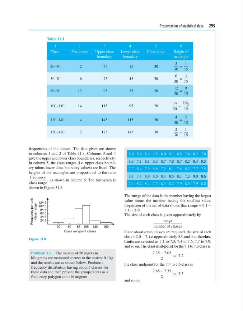
frequencies of the classes. The data given are shown
in columns 1 and 2 of Table 31.3. Columns 3 and 4
give the upper and lower class boundaries, respectively.
In column 5, the class ranges (i.e. upper class boundary minus lower class boundary values) are listed. The
heights of the rectangles are proportional to the ratio
frequency
class range
, as shown in column 6. The histogram is
shown in Figure 31.8.
30
4/15
2/15
6/15
Frequency per unit
class range
10/15
8/15
12/15
60
85
Class mid-point values
130
160
105
Figure 31.8
Problem 12. The masses of 50 ingots in
kilograms are measured correct to the nearest 0.1 kg
and the results are as shown below. Produce a
frequency distribution having about 7 classes for
these data and then present the grouped data as a
frequency polygon and a histogram
8.0 8.6 8.2 7.5 8.0 9.1 8.5 7.6 8.2 7.8
8.3 7.1 8.1 8.3 8.7 7.8 8.7 8.5 8.4 8.5
7.7 8.4 7.9 8.8 7.2 8.1 7.8 8.2 7.7 7.5
8.1 7.4 8.8 8.0 8.4 8.5 8.1 7.3 9.0 8.6
7.4 8.2 8.4 7.7 8.3 8.2 7.9 8.5 7.9 8.0
The range of the data is the member having the largest
value minus the member having the smallest value.
Inspection of the set of data shows that range = 9.1 −
7.1 = 2.0.
The size of each class is given approximately by
range
number of classes
Since about seven classes are required, the size of each
class is 2.0 ÷ 7, i.e. approximately 0.3, and thus the class
limits are selected as 7.1 to 7.3, 7.4 to 7.6, 7.7 to 7.9,
and so on. The class mid-point for the 7.1 to 7.3 class is
7.35 + 7.05
2
i.e. 7.2
the class midpoint for the 7.4 to 7.6 class is
7.65 + 7.35
2
i.e. 7.5
and so on.
Table 31.3
1
2
3
4
5
6
Class
Frequency
Upper class
Lower class
Class range
Height of
boundary
boundary
rectangle
20–40
2
45
15
30
2
30
=
1
15
50–70
6
75
45
30
6
30
=
3
15
80–90
12
95
75
20
12
20
=
9
15
100–110
14
115
95
20
14
20
=
10
1
2
15
120–140
4
145
115
30
4
30
=
2
15
150–170
2
175
145
30
2
30
=
1
15
frequencies of the classes. The data given are shown
in columns 1 and 2 of Table 31.3. Columns 3 and 4
give the upper and lower class boundaries, respectively.
In column 5, the class ranges (i.e. upper class boundary minus lower class boundary values) are listed. The
heights of the rectangles are proportional to the ratio
frequency
class range
, as shown in column 6. The histogram is
shown in Figure 31.8.
30
4/15
2/15
6/15
Frequency per unit
class range
10/15
8/15
12/15
60
85
Class mid-point values
130
160
105
Figure 31.8
Problem 12. The masses of 50 ingots in
kilograms are measured correct to the nearest 0.1 kg
and the results are as shown below. Produce a
frequency distribution having about 7 classes for
these data and then present the grouped data as a
frequency polygon and a histogram
8.0 8.6 8.2 7.5 8.0 9.1 8.5 7.6 8.2 7.8
8.3 7.1 8.1 8.3 8.7 7.8 8.7 8.5 8.4 8.5
7.7 8.4 7.9 8.8 7.2 8.1 7.8 8.2 7.7 7.5
8.1 7.4 8.8 8.0 8.4 8.5 8.1 7.3 9.0 8.6
7.4 8.2 8.4 7.7 8.3 8.2 7.9 8.5 7.9 8.0
The range of the data is the member having the largest
value minus the member having the smallest value.
Inspection of the set of data shows that range = 9.1 −
7.1 = 2.0.
The size of each class is given approximately by
range
number of classes
Since about seven classes are required, the size of each
class is 2.0 ÷ 7, i.e. approximately 0.3, and thus the class
limits are selected as 7.1 to 7.3, 7.4 to 7.6, 7.7 to 7.9,
and so on. The class mid-point for the 7.1 to 7.3 class is
7.35 + 7.05
2
i.e. 7.2
the class midpoint for the 7.4 to 7.6 class is
7.65 + 7.35
2
i.e. 7.5
and so on.