

156 Basic Engineering Mathematics
Rearranging each equation into y = mx + c form gives
y = −1.20x + 1.80
(1)
y =
x
5.0
−
8.5
5.0
i.e.
y = 0.20x − 1.70
(2)
Three co-ordinates are calculated for each equation as
shown below.
x
0
1
2
y = −1.20x + 1.80
1.80
0.60
−0.60
x
0
1
2
y = 0.20x − 1.70 −1.70 −1.50 −1.30
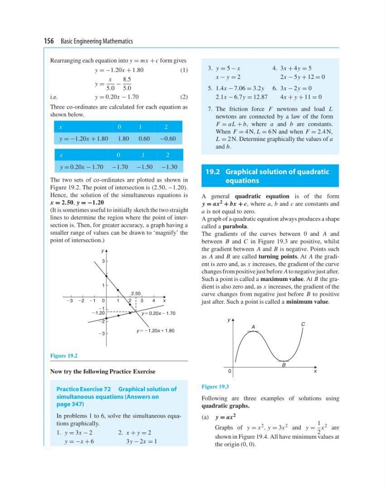
The two sets of co-ordinates are plotted as shown in
Figure 19.2. The point of intersection is (2.50, −1.20).
Hence, the solution of the simultaneous equations is
x = 2.50, y = −1.20
(It is sometimes useful to initially sketch the two straight
lines to determine the region where the point of intersection is. Then, for greater accuracy, a graph having a
smaller range of values can be drawn to ‘magnify’ the
point of intersection.)
21
21
22
23
21.20
22
23
3
1
0
1
2
3
2.50
4
y
x
y 5 0.20x 2 1.70
y 5 21.20x 1 1.80
Figure 19.2
Now try the following Practice Exercise
Practice Exercise 72 Graphical solution of
simultaneous equations (Answers on
page 347)
In problems 1 to 6, solve the simultaneous equations graphically.
1. y = 3x − 2
2 . x + y = 2
y = −x + 6
3 y − 2x = 1
3. y = 5 − x
4. 3x + 4y = 5
x − y = 2
2 x − 5y + 12 = 0
5. 1.4x − 7.06 = 3.2y 6. 3x − 2y = 0
2.1x − 6.7y = 12.87
4x + y + 11 = 0
7. The friction force F newtons and load L
newtons are connected by a law of the form
F = aL + b, where a and b are constants.
When F = 4 N, L = 6 N and when F = 2.4 N,
L = 2 N. Determine graphically the values of a
and b.
19.2 Graphical solution of quadratic
equations
A general quadratic equation is of the form
y = ax 2 + bx + c, where a, b and c are constants and
a is not equal to zero.
A graph of a quadratic equation always produces a shape
called a parabola.
The gradients of the curves between 0 and A and
between B and C in Figure 19.3 are positive, whilst
the gradient between A and B is negative. Points such
as A and B are called turning points. At A the gradient is zero and, as x increases, the gradient of the curve
changes from positive just before A to negative just after.
Such a point is called a maximum value. At B the gradient is also zero and, as x increases, the gradient of the
curve changes from negative just before B to positive
just after. Such a point is called a minimum value.
y
x
A
C
B
0
Figure 19.3
Following are three examples of solutions using
quadratic graphs.
(a) y = ax 2
Graphs of y = x 2 , y = 3x 2 and y =
1
2
x 2 are
shown in Figure 19.4. All have minimum values at
the origin (0, 0).
Rearranging each equation into y = mx + c form gives
y = −1.20x + 1.80
(1)
y =
x
5.0
−
8.5
5.0
i.e.
y = 0.20x − 1.70
(2)
Three co-ordinates are calculated for each equation as
shown below.
x
0
1
2
y = −1.20x + 1.80
1.80
0.60
−0.60
x
0
1
2
y = 0.20x − 1.70 −1.70 −1.50 −1.30
The two sets of co-ordinates are plotted as shown in
Figure 19.2. The point of intersection is (2.50, −1.20).
Hence, the solution of the simultaneous equations is
x = 2.50, y = −1.20
(It is sometimes useful to initially sketch the two straight
lines to determine the region where the point of intersection is. Then, for greater accuracy, a graph having a
smaller range of values can be drawn to ‘magnify’ the
point of intersection.)
21
21
22
23
21.20
22
23
3
1
0
1
2
3
2.50
4
y
x
y 5 0.20x 2 1.70
y 5 21.20x 1 1.80
Figure 19.2
Now try the following Practice Exercise
Practice Exercise 72 Graphical solution of
simultaneous equations (Answers on
page 347)
In problems 1 to 6, solve the simultaneous equations graphically.
1. y = 3x − 2
2 . x + y = 2
y = −x + 6
3 y − 2x = 1
3. y = 5 − x
4. 3x + 4y = 5
x − y = 2
2 x − 5y + 12 = 0
5. 1.4x − 7.06 = 3.2y 6. 3x − 2y = 0
2.1x − 6.7y = 12.87
4x + y + 11 = 0
7. The friction force F newtons and load L
newtons are connected by a law of the form
F = aL + b, where a and b are constants.
When F = 4 N, L = 6 N and when F = 2.4 N,
L = 2 N. Determine graphically the values of a
and b.
19.2 Graphical solution of quadratic
equations
A general quadratic equation is of the form
y = ax 2 + bx + c, where a, b and c are constants and
a is not equal to zero.
A graph of a quadratic equation always produces a shape
called a parabola.
The gradients of the curves between 0 and A and
between B and C in Figure 19.3 are positive, whilst
the gradient between A and B is negative. Points such
as A and B are called turning points. At A the gradient is zero and, as x increases, the gradient of the curve
changes from positive just before A to negative just after.
Such a point is called a maximum value. At B the gradient is also zero and, as x increases, the gradient of the
curve changes from negative just before B to positive
just after. Such a point is called a minimum value.
y
x
A
C
B
0
Figure 19.3
Following are three examples of solutions using
quadratic graphs.
(a) y = ax 2
Graphs of y = x 2 , y = 3x 2 and y =
1
2
x 2 are
shown in Figure 19.4. All have minimum values at
the origin (0, 0).