

152 Basic Engineering Mathematics
From para (a), page 150, if T = kL
n
then
lg T = n lg L + lg k
and comparing with
Y = m X + c
shows that lg T is plotted vertically against lg L horizontally, with gradient n and vertical-axis intercept
lg k.
A table of values for lg T and lg L is drawn up as shown
below.
T
1.0
1.3
1.5
1.8
2.0
2.3
lg T 0
0.114 0.176 0.255 0.301 0.362
L
0.25
0.42
0.56
0.81 1.0
1.32
lg L −0.602 −0.377 −0.252 −0.092 0
0.121
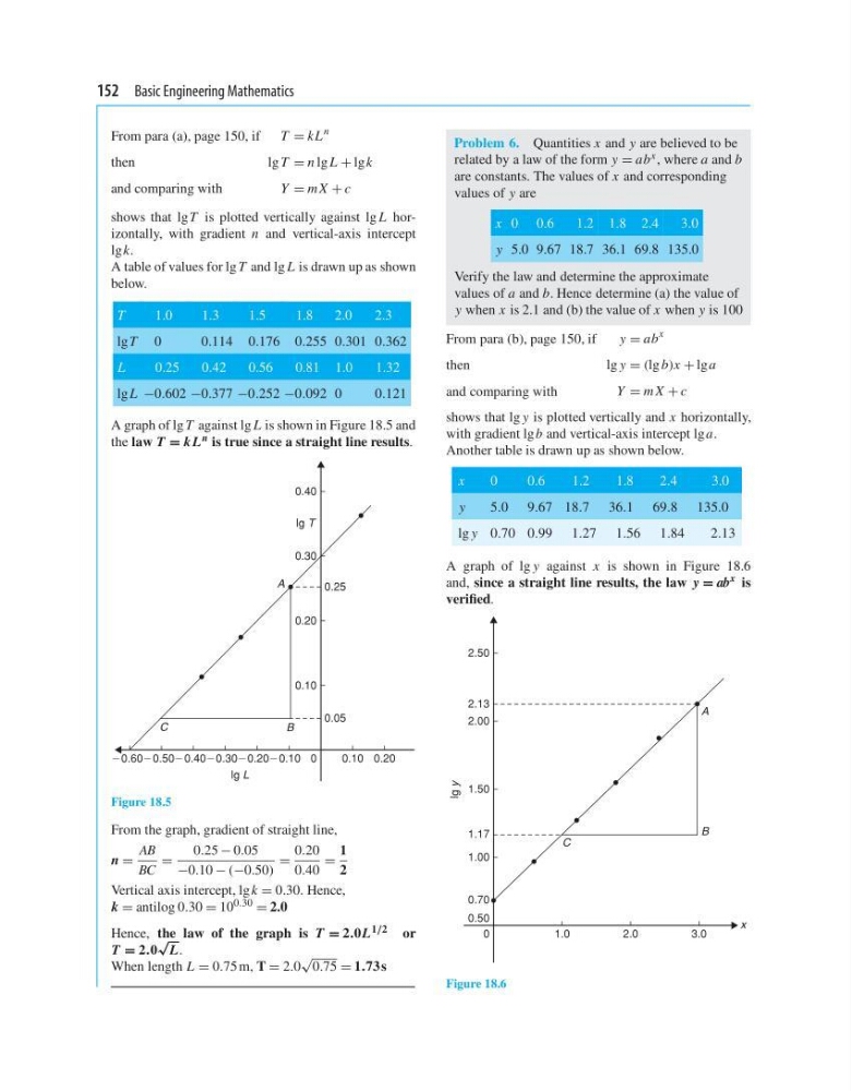
A graph of lg T against lg L is shown in Figure 18.5 and
the law T = kL n is true since a straight line results.
A
B
C
0
20.40
20.50
20.60
20.3020.20
0.20
0.10
0.20
0.30
0.25
0.05
lg L
lg T
0.40
20.10
0.10
Figure 18.5
From the graph, gradient of straight line,
n =
AB
BC
=
0.25 − 0.05
−0.10 − (−0.50)
=
0.20
0.40
=
1
2
Vertical axis intercept, lg k = 0.30. Hence,
k = antilog 0.30 = 10 0.30 = 2.0
Hence, the law of the graph is T = 2.0L 1/2 or
T = 2.0
√
L.
When length L = 0.75 m, T = 2.0
√
0.75 = 1.73 s
Problem 6. Quantities x and y are believed to be
related by a law of the form y = ab x , where a and b
are constants. The values of x and corresponding
values of y are
x 0 0.6
1.2 1.8 2.4
3.0
y 5.0 9.67 18.7 36.1 69.8 135.0
Verify the law and determine the approximate
values of a and b. Hence determine (a) the value of
y when x is 2.1 and (b) the value of x when y is 100
From para (b), page 150, if
y = ab
x
then
lg y = (lg b)x + lg a
and comparing with
Y = m X + c
shows that lg y is plotted vertically and x horizontally,
with gradient lg b and vertical-axis intercept lg a.
Another table is drawn up as shown below.
x
0
0.6
1.2
1.8
2.4
3.0
y
5.0 9.67 18.7 36.1 69.8 135.0
lg y 0.70 0.99 1.27 1.56 1.84
2.13
A graph of lg y against x is shown in Figure 18.6
and, since a straight line results, the law y = ab
x is
verified.
C
B
A
lg y
x
2.50
2.13
2.00
1.50
1.00
1.17
0.50
0
1.0
2.0
3.0
0.70
Figure 18.6
From para (a), page 150, if T = kL
n
then
lg T = n lg L + lg k
and comparing with
Y = m X + c
shows that lg T is plotted vertically against lg L horizontally, with gradient n and vertical-axis intercept
lg k.
A table of values for lg T and lg L is drawn up as shown
below.
T
1.0
1.3
1.5
1.8
2.0
2.3
lg T 0
0.114 0.176 0.255 0.301 0.362
L
0.25
0.42
0.56
0.81 1.0
1.32
lg L −0.602 −0.377 −0.252 −0.092 0
0.121
A graph of lg T against lg L is shown in Figure 18.5 and
the law T = kL n is true since a straight line results.
A
B
C
0
20.40
20.50
20.60
20.3020.20
0.20
0.10
0.20
0.30
0.25
0.05
lg L
lg T
0.40
20.10
0.10
Figure 18.5
From the graph, gradient of straight line,
n =
AB
BC
=
0.25 − 0.05
−0.10 − (−0.50)
=
0.20
0.40
=
1
2
Vertical axis intercept, lg k = 0.30. Hence,
k = antilog 0.30 = 10 0.30 = 2.0
Hence, the law of the graph is T = 2.0L 1/2 or
T = 2.0
√
L.
When length L = 0.75 m, T = 2.0
√
0.75 = 1.73 s
Problem 6. Quantities x and y are believed to be
related by a law of the form y = ab x , where a and b
are constants. The values of x and corresponding
values of y are
x 0 0.6
1.2 1.8 2.4
3.0
y 5.0 9.67 18.7 36.1 69.8 135.0
Verify the law and determine the approximate
values of a and b. Hence determine (a) the value of
y when x is 2.1 and (b) the value of x when y is 100
From para (b), page 150, if
y = ab
x
then
lg y = (lg b)x + lg a
and comparing with
Y = m X + c
shows that lg y is plotted vertically and x horizontally,
with gradient lg b and vertical-axis intercept lg a.
Another table is drawn up as shown below.
x
0
0.6
1.2
1.8
2.4
3.0
y
5.0 9.67 18.7 36.1 69.8 135.0
lg y 0.70 0.99 1.27 1.56 1.84
2.13
A graph of lg y against x is shown in Figure 18.6
and, since a straight line results, the law y = ab
x is
verified.
C
B
A
lg y
x
2.50
2.13
2.00
1.50
1.00
1.17
0.50
0
1.0
2.0
3.0
0.70
Figure 18.6