15.1014
68.7896
75.1904
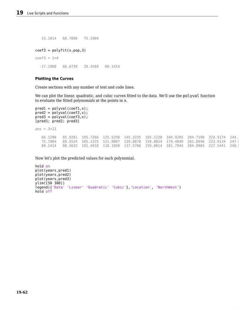
coef3 = polyfit(x,pop,3)
coef3 = 1×4
-17.1908
66.6739
29.4569
80.1414
Plotting the Curves
Create sections with any number of text and code lines.
We can plot the linear, quadratic, and cubic curves fitted to the data. We'll use the polyval function
to evaluate the fitted polynomials at the points in x.
pred1 = polyval(coef1,x);
pred2 = polyval(coef2,x);
pred3 = polyval(coef3,x);
[pred1; pred2; pred3]
ans = 3×11
66.1296
85.9281 105.7266 125.5250 145.3235 165.1220 184.9205 204.7190 224.5174 244.3
75.1904
89.5524 105.1225 121.9007 139.8870 159.0814 179.4840 201.0946 223.9134 247.9
80.1414
88.5622 101.4918 118.1050 137.5766 159.0814 181.7944 204.8904 227.5441 248.9
Now let's plot the predicted values for each polynomial.
hold on
plot(years,pred1)
plot(years,pred2)
plot(years,pred3)
ylim([50 300])
legend({'Data' 'Linear' 'Quadratic' 'Cubic'},'Location', 'NorthWest')
hold off
19 Live Scripts and Functions
19-62