Chapter 70
A numerical method of
harmonic analysis
70.1 Introduction
Many practical waveforms can be represented by simple mathematical expressions, and, by using Fourier
series, the magnitude of their harmonic components
determined, as shown in Chapters 66 to 69. For waveforms not in this category, analysis may be achieved by
numerical methods. Harmonic analysis is the process
of resolving a periodic, non-sinusoidal quantity into a
series of sinusoidal components of ascending order of
frequency.
70.2 Harmonic analysis on data given
in tabular or graphical form
The Fourier coefficients a 0 , a n and b n used in Chapters 66 to 69 all require functions to be integrated, i.e.
a 0 =
1
2π
π
−π
f (x)dx =
1
2π
2π
0
f (x) dx
= mean value of f (x)
in the range−π to π or 0 to 2π
a n =
1
π
π
−π
f (x) cos nx dx
=
1
π
2π
0
f (x) cos nx dx
= twice the mean value of f (x) cos nx
in the range 0 to 2π
b n =
1
π
π
−π
f (x) sin nx dx
=
1
π
2π
0
f (x) sin nx dx
= twice the mean value of f (x) sin nx
in the range 0 to 2π
However, irregular waveforms are not usually defined
by mathematical expressions and thus the Fourier coefficients cannot be determined by using calculus. In these
cases, approximate methods, such as the trapezoidal
rule, can be used to evaluate the Fourier coefficients.
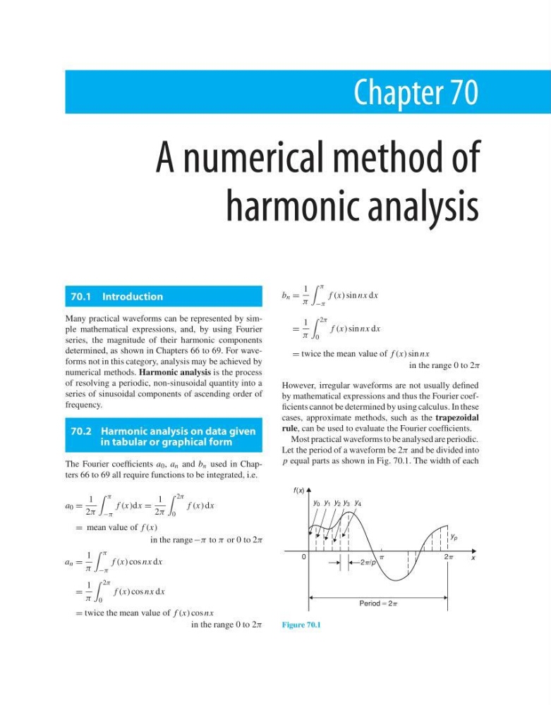
Most practical waveforms to be analysed are periodic.
Let the period of a waveform be 2π and be divided into
p equal parts as shown in Fig. 70.1. The width of each
f(x)
0
Period 5 2␲
2␲/p
2␲
x
y p
␲
y 0 y 1 y 2 y 3 y 4
Figure 70.1